Predicting Ancestry Using mtDNA

Introduction

Imagine you have two complete mtDNA genomes, A and B, and you’d like to determine which one of the two is the ancestor of the other, with no other information whatsoever. This is simply impossible to determine, since they have only a single, mutual relationship with each other, which consists of some number of bases in common. Yes, of course, if you have access to other information about where in history certain genes or other genome regions fall, or other information concerning the provenance of the genomes, then you might be able to actually date the genomes. However, the point is, that in the absence of information exogenous to the two genomes, you simply cannot determine which of the two is the ancestor of the other, given only the raw genome sequences themselves.

Now assume instead you’re given three genomes, A, B, and C, where all three genomes are from distinct populations. Further, assume that it is in fact the case that genome A comes from the ethnic ancestor population of genomes B and C. Note that this does not require genome A to be older than genomes B and C, and in fact, all genomes could have been sourced from living persons. The point is instead that genomes B and C are literally mutations of genome A. It follows that it is far more likely that genomes B and C have less in common with each other, than either of them do with genome A. To assume otherwise implies that genomes B and C developed even more common bases over time simply by chance. It is instead far more likely that mutations over time cause B and C to diverge along separate paths of mutation. For intuition, imagine that two people are tossing independent and unbiassed coins. Further, assume that by chance, they happen to both throw three heads in a row. From that point going forward, they are almost certainly going to diverge along two different paths of outcomes, and as the number of coin tosses increases, the probability of both throwing exactly the same sequence starts to decrease rapidly. Therefore, if we assume that A is the common ancestor of both B and C, then it is most likely that A has more bases in common with both B and C, than B and C have in common with each other.

This is a very simple condition to test for, which reduces to a simple inequality. Specifically, let denote the set of bases genomes A and B have in common. We can then write to denote the cardinality of the set of common bases, which is simply the number of bases A and B have in common. Returning to the condition above, if it is in fact the case that genome A is the ancestor of genomes B and C, then it is almost certainly the case that and . Again, this simply means that genomes B and C have fewer bases in common with each other, than either of them do with A, which is again the most likely outcome if B and C are in fact mutations of A.

However, this does not tell you how long ago the mutations occurred, and because mtDNA is at times incredibly stable, over thousands of years, you simply can’t claim an amount of time has lapsed that generated the observed mutations. It is instead a simply ordinal relationship, that again does not imply ancestry, but is instead consistent with ancestry. As a consequence, the most narrow interpretation is that all relationships that fail this test almost certainly rule out ancestry. Nonetheless, the results produced are consistent with known history and common sense.

Application to Data

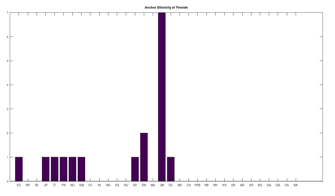
Below is the graph produced by analyzing the Kazakh genomes in the dataset linked to at the end of this article. A given vertex is attached to another pair, if they satisfy the inequality above. The graphs are automatically generated by the attached Octave code below, using SageMath, you just need to copy / paste the SageMath code, which is written to a file. As you can plainly see, the Kazakh people are a cradle of humanity, and in fact, this is consistent with known history, as Homo sapiens have been in Kazakhstan for hundreds of thousands of years. The vertex labels on the graph are the genome row numbers in the dataset, and the color key to the right tells you to which population a given genome belongs.

There are some other examples that superficially seem to go the wrong way in time, but this is incorrect. Specifically, if you run this analysis on the Mexican genomes, you find that one of the Mexican genomes is the ancestor of a Chachapoya genome, which is plainly ancient. But there’s nothing unusual about this at all, because it could of course be the case that the Mexican individual is the living representative of a people that predated and are the ancestors of the Chachapoyas. This is possible because mtDNA is so stable. Note that because the dataset has been diligenced to ensure provenance, if a genome is e.g., identified as Mexican, then the individual in question is ethnically Mexican, as opposed to simply located in Mexico (see Technical Notes below).

Technical Notes

I’ll begin by explaining in more detail how the algorithm actually works, and then close with some notes on the provenance of the dataset itself. As noted above, the core test is satisfaction of a simple inequality between three genomes. However, the algorithm has some optimization in it. Specifically, it begins by building clusters for each genome of the dataset, where a genome B is included in the cluster for genome A if genomes A and B have at least 99% of their bases in common. This builds a cluster of 99% matches for every genome in the dataset. It then fixes a genome C, and searches for the genome B, that minimizes the number of bases in common. Assume that genome B is found in the cluster for genome A. It then tests the inequality, which if satisfied, ensures that genomes A and B, and A and C, have more bases in common than genomes B and C. However, it also ensures that genomes A and B, and A and C, are a 99% match, and moreover, genome B minimizes the number of matching bases between B and C, over the entire dataset. As a consequence, this algorithm ensures that genomes A and B, and A and C, are a 99% match, and at the same time, ensures the maximum amount of mutation has occurred separating genomes B and C. Said otherwise, this ensures that genomes B and C are as dissimilar as possible, given the dataset, yet both mutually connected to another genome A, with which both have a 99% match. Finally, the code ensures that the result is either a tree, or a collection of trees (i.e., a forest), in that it precludes loops, and precludes parents from being linked to by children (note that the graphs are directed).

The dataset itself consists of 382 complete human mtDNA genomes from the NIH Database, taken from 33 ethnicities, including several ancient and archaic ethnicities. All of the genomes have been diligenced to ensure that the GenBank notes associated with the genomes imply the actual ethnicities, as opposed to just the location of the individual. That is, if the classifier for a genome is e.g., Chinese, then the GenBank notes explicitly state or plainly suggest that the sample is in fact from an ethnically Chinese person, as opposed to a person located in China.

The method of comparison involves counting matching bases, after a simple alignment that shifts the entire genome (if at all), to align it to what is plainly a globally common sequence of 15 bases. This is also apparently the default NIH alignment, which you can see for yourself by looking through their database. See e.g., these three genomes: Genome 1, Genome 2, and Genome 3, all of which contain exactly the same opening 15 characters. Because mtDNA is circular, this is plainly a deliberate starting point that we use as well, for simplicity. Finally, note that most of the genomes do not need to be shifted at all, because the NIH presents nearly all of the genomes I’ve seen using exactly the same alignment. Specifically, only 5 out of the 382 genomes in the dataset were shifted by an average of 2 bases.

The only thing I’ve learned studying genetics, is that nothing we think of is true in terms of race, and that all of our mothers, are probably severely disappointed in us.

Here’s the code:

https://www.dropbox.com/s/pmi56hjjugzcwrk/Generate_Heridity_Tree.m?dl=0

https://www.dropbox.com/s/1ikhuz6xnaesejh/Genetic_Furthest_Neighbor_Single_Row.m?dl=0

https://www.dropbox.com/s/y19d8ein5wjxe3a/Genetic_Alignment.m?dl=0

https://www.dropbox.com/s/nrczoxeqezvnls1/Genetic_Preprocessing.m?dl=0

https://www.dropbox.com/s/aeko80flttnk8b3/Genetic_ShiftbyK.m?dl=0

Here’s the dataset:

https://www.dropbox.com/s/8jlwr49fhtstpre/mtDNA.zip?dl=0

Measuring the Diversity of Global Maternal Lines

Introduction

In a previous article, I showed that there are only 6 maternal lines that are a 99% match to 67.64% of global maternal lines, using a dataset of 377 complete mtDNA genomes, from 32 ethnicities. This suggests, that as a general matter, human beings are already extremely diverse, since a majority of the global population can be traced back to just a handful of maternal lines. There’s still the question of how we should measure this, and in this article, I’ll present a few methods that will allow us to quantify exactly how diverse a given population is.

Counting the Number of Maternal Lines in a Population

In the previous article, we counted the number of global maternal lines by building mutually exclusive clusters over the entire dataset of 377 genomes. This was done by first building a cluster of 99% matches for each genome in the dataset. That is, for a given genome A, if genome B has 99% of its bases in common with genome A, then genome B is included in the cluster for Genome A. We then sort the clusters by size, beginning with the largest cluster, and allocating all of the genomes in the largest cluster to that cluster, and removing them from all others. We then do this for the next largest cluster, and so on. This eventually produces mutually exclusive clusters.

If we limit this process to a given population, we will create mutually exclusive clusters that all belong to the same population. For example, if we begin with all of the Japanese genomes, and then apply this process, we will produce mutually exclusive clusters, each of which consists of genomes that are a 99% match to some given genome. As a consequence, this will partition a given population into distinct maternal lines, with each cluster containing genomes that are part of a distinct maternal line within the population in question. The table below shows the total number of genomes in each population, the number of clusters (i.e., distinct maternal lines) in each population, and the average cluster size, for each of the 32 population ethnicities. As you can see, the only truly homogenous populations are the Kazakh, Nepalese, and Iberian Roma, whereas everyone else is fairly heterogenous. 

Ethnicity	No. Genomes	No. Clusters	Avg. Cluster Size
1. Kazakh	30	6	5.00
2. Nepalese	20	3	6.67
3. Iberian Roma	19	1	19.00
4. Japanese	20	10	2.00
5. Italian	19	10	1.90
6. Finnish	20	13	1.54
7. Norwegian	20	9	2.22
8. Swedish	20	8	2.12
9. Chinese	20	12	1.67
10. Indian	18	7	2.57
11. Nigerian	9	6	1.50
12. Egyptian	20	8	2.50
13. Russian	6	3	2.00
14. Spanish	13	9	1.44
15. Danish	9	5	1.80
16. Maritime Archaic	10	6	1.67
17. Ashkenazi Jewish	18	6	3.00
18. Scottish	18	10	1.80
19. Mexican	3	3	1.00
20. Chachapoya	10	6	1.67
21. Pre-Roman Egyptian (4,000 B.P.)	1	1	1.00
22. Homo Heidelbergensis	1	1	1.00
23. Mayan	10	4	2.50
24. Khoisan	10	10	1.00
25. English	9	7	1.29
26. Ancient Roman	5	2	2.50
27. Sardinian	5	2	2.50
28. Basque	4	2	2.00
29. Georgian	2	2	1.00
30. German	9	7	1.29
31. Denisovan	1	1	1.0
32. Neanderthal	1	1	1.0

Measuring the Global Reach of a Population

We can apply a similar process for a selected population over the entire dataset. That is, we first take all of the genomes in a given selected population, and then build clusters by finding all other genomes, over all populations, that are a 99% match with a given genome from the selected population. We then build mutually exclusive clusters in the exact same manner we did above, first sorting by cluster size, and then allocating the matching genomes in size order. This will allow us to find the breadth of global populations that match to a given genome from the selected population, and will again partition the population, because not all genomes from the selected population will produce non-empty clusters. However, in this case, we will consider every non-empty cluster, rather than impose a minimum size. This will allow us to distinguish between a population that is simply heterogenous, as opposed to global. For example, Nigerians are heterogenous in that they have numerous maternal lines, however only one of the maternal lines is truly global, which shows a plain connection to Northern Europeans, Norwegians and Scotts in particular. It’s tempting to write these connections off due to the slave trade, but this just doesn’t really hold up in the case of Japan and China, or even more peculiar, Kazakstan and the Chachapoyas. The bottom line is that an ethnically Nigerian maternal line is a basically perfect match for the ethnicities below, which does not have a simple explanation in known history (to my knowledge). In my opinion, it makes much more sense to instead assume that truly inexplicable cases like these are due to ancient migration patterns that are still observable today, simply because mtDNA doesn’t change much over time, and in some cases, enormous periods of time.

The y-axis shows the number of matching genomes from a given population, and the x-axis shows the population acronym.

Applying this to the Japanese population, this produces 11 clusters, with a total of 210 genomes, or 56% of the dataset, which suggests that the Japanese maternal line is quite global, despite the reputation of being an insular nation. It turns out that Japan is only recently insular, as it started in the 1600’s in response to Spanish, Portuguese, and Catholic attempts to impose colonial rule, and even enslave Japanese people. This of course leaves open the rest of human history, which is hundreds of thousands of years old, providing plenty of opportunity for the diversity that is obviously present in literally every population, other than the Kazakhs, Roma, and Nepalese people. In the case of the Japanese, you see a simply incredible scope of global populations, and below are the most interesting clusters I noticed. Among them is a Japanese genome that is a perfect match for 6 out of the 10 Ancient Mayan genomes, and nothing else, suggesting the individual in question is quite literally of Ancient Mayan heritage.

The y-axis shows the number of matching genomes from a given population, and the x-axis shows the population acronym.

Keep in mind the dataset has been diligenced to ensure that the GenBank notes either explicitly state or plainly suggest that the person in question is of the ethnicity in question. Moreover, there’s a link for each genome to the NIH Database, where you can check the provenance yourself. So if e.g., a genome is classified as Japanese, then the GenBank notes indicate that the person is ethnically Japanese, as opposed to the genome simply being collected from a person in Japan. Because of this, and the 99% threshold, you simply cannot argue with these results: humanity is already extremely diverse, suggesting a rich and ancient history that is arguably unknown to us, that will probably be discoverable at least initially only through genetics, rather than archaeology. Because mtDNA is so stable over time, it makes perfect sense as the initial point of inquiry.

Again, the only things you need to allow for expansive global trade are sailboats and telescopes, and the bottom line is, the people of Polynesia got there somehow, and they certainly didn’t use unguided rowboats. Moreover, the Ancient Romans had glass, and careful observation of optics through water would suggest that vision can be adjusted using materials, including of course glass, which was plainly known to at least one ancient civilization. Finally, below is a table that shows the number of genomes per population, together with the applicable acronym used in the charts above, and below that is the dataset and command line code.

Ethnicity	Genome Count	Abbreviation
1. Kazakh	30	KZ
2. Nepalese	20	NP
3. Iberian Roma	19	IB
4. Japanese	20	JP
5. Italian	19	IT
6. Finnish	20	FN
7. Norwegian	20	NO
8. Swedish	20	SW
9. Chinese	20	CC
10. Indian	18	IN
11. Nigerian	9	NG
12. Egyptian	20	EG
13. Russian	6	RU
14. Spanish	13	SP
15. Danish	9	DN
16. Maritime Archaic	10	MA
17. Ashkenazi Jewish	18	JW
18. Scottish	18	SC
19. Mexican	3	MX
20. Chachapoya	10	CH
21. Pre-Roman Egyptian (4,000 B.P.)	1	PRE
22. Homo Heidelbergensis	1	HB
23. Mayan	10	MY
24. Khoisan	10	KH
25. English	9	EN
26. Ancient Roman	5	AR
27. Sardinian	5	SR
28. Basque	4	BQ
29. Georgian	2	GA
30. German	9	GR
31. Denisovan	1	DS
32. Neanderthal	1	NA

Here’s the dataset:

https://www.dropbox.com/s/8jlwr49fhtstpre/mtDNA.zip?dl=0

Here’s the command line code:

https://www.dropbox.com/s/4v1fo2hkt76pjws/Count%20Unique%20Population%20Genomes.m?dl=0

https://www.dropbox.com/s/hi1ggfgqnat1dwo/Mut_Exc_Clusters_By_Class.m?dl=0

VeGa

Attached is an updated draft of my book VeGa.

Enjoy!

VeGa

The Distribution of Archaic mtDNA

Introduction

We know that many living humans carry archaic DNA, specifically people in Iceland and Polynesia, and likely many others. However, mtDNA is inherited from one generation to the next along the maternal line, with almost no mutations. As a consequence, if there is any nexus between archaic humans and modern humans, then that nexus should be strongest along the maternal line, specifically, as captured by mtDNA. As it turns out, many modern humans globally are a near perfect match on their maternal line for Homo heidelbergensis, and some are a good match for Denisovans.

Technical Notes

I’ve assembled a dataset of 377 complete human mtDNA genomes from the NIH Database, taken from 32 ethnicities, including several ancient and archaic ethnicities. All of the genomes have been diligenced to ensure that the GenBank notes associated with the genomes imply the actual ethnicities, as opposed to just the location of the individual. That is, if the classifier for a genome is Chinese, then the GenBank notes explicitly state or plainly suggest that the sample is in fact from an ethnically Chinese person, as opposed to a genome collected in China. The dataset includes one complete Homo heidelbergensis genome, and one complete Denisovan genome.

The method of comparison involves counting matching bases, after a simple alignment that shifts the entire genome (if at all), to align it to what is plainly a globally common sequence of 15 bases. This is also apparently the default NIH alignment, which you can see for yourself by looking through their database. See e.g., these three genomes: Genome 1, Genome 2, and Genome 3, all of which contain exactly the same opening 15 characters. Because mtDNA is circular, this is plainly a deliberate starting point that we use as well, for simplicity. Finally, note that most of the genomes do not need to be shifted at all, because the NIH presents nearly all of the genomes I’ve seen using exactly the same alignment. Specifically, only 5 out of the 377 genomes in the dataset were shifted by an average of 2 bases.

As a consequence, I do not account for insertions and deletions outside of the opening sequence, and this is deliberate, since insertions and deletions are associated with drastic changes in behaviors and morphologies, in contrast to point mutations. For example, both Down Syndrome and Williams Syndrome are the result of insertions and deletions, and they both produce drastic behavioral and morphological changes. As a consequence, the method I employ is much more stringent than e.g., the one employed by NIH Blast, which will segment a genome and look for local alignments that maximize matching bases. That is, if two genomes produce e.g., a 99% match in the method I use, then they really are a 99% match over the entire genome, unadjusted, save for any shifting necessary to align the genomes to a common opening sequence of 15 bases, which again is unnecessary for the vast majority of genomes. Finally, note that the Heidelbergensis and Denisovan genomes were not shifted at all during the alignment process, and again, only 1.326% of the dataset required shifting.

Application to Data

We begin by simply plotting the number of matching bases between the Heidelbergensis and Denisovan genomes, and the entire dataset. Both plots are shown below. As you can see, the number of individuals that are a strong match with Heidelbergensis exceeds the number of individuals that are a strong match to Denisovan. Moreover, the match count is also plainly higher for Heidelbergensis, suggesting that many people are a near-perfect match to Heidelbergensis, whereas only some people are a strong match to Denisovan.

The y-axis shows the number of matching bases between a given genome and Heidelbergensis (left) and Denisovan (right), and the x-axis shows the genome index in the dataset.

We can conduct similar analysis by population ethnicity, and we’ll begin with Heidelbergensis, setting the minimum match percentage to 96%, and then counting the number of genomes in each population that are a 96% match to Heidelbergensis. This is shown in the plot below. Note that a minimum match percentage of 97% produces an empty set, and so 96% is the maximum whole-number percentage that produces a non-empty set. Therefore, the populations below represent some of the strongest matches to Heidelbergensis. The population names and their corresponding acronyms can be found in a table at the end of the article. Also note that the number of genomes per population is not uniform, and can also be found in the same table below. As you can see, the matches are concentrated in the Kazakh and Roma populations, which contain 30 and 19 genomes, respectively, in the full dataset. This implies that 73% of Kazakh and 100% of Roma are likely direct descendants of Heidelbergensis. The distribution below contains a total of 72 genomes, suggesting that 19% of the global population are direct descendants of Heidelbergensis.

The y-axis shows the number of matching genomes between Heidelbergensis and a given population, and the x-axis shows the population acronym.

We can conduct the exact same analysis for Denisovan, however as noted above, the match count is not as strong. Specifically, a minimum match percentage of 74% produces an empty set, 73% produces exactly one Finnish genome, and 72% produces a global distribution that contains 25 genomes, which is shown below. As you can see, the distribution is concentrated in the Finnish and Ashkenazi Jewish populations, which contain 20 and 18 genomes, respectively, in the full dataset. This implies that 25% of Finns and 44% of Ashkenazi Jews are closely related to Denisovans. Again, this distribution contains 25 genomes, suggesting that 7% of the global population are closely related to Denisovans.

The y-axis shows the number of matching bases between a given genome and Denisovan, and the x-axis shows the genome index in the dataset.

Comparison to the Global Population

As demonstrated above, many modern humans are closely related to archaic humans on the maternal line. This makes perfect sense, since we know that Homo sapiens mated with archaic humans. Because this is known to have occurred, and because mtDNA is transmitted from one generation to the next without much (if any) mutation, it follows that at least some modern humans should be closely related to archaic humans, which seems to be the case, with 24% of the dataset either directly descended from or closely related to an archaic human.

The y-axis shows the number of matching bases between a given remaining genome and Heidelbergensis, and the x-axis shows the genome index in the dataset.

We can further analyze how much mtDNA the rest of the global population has in common with both Heidelbergensis and Denisovans. Note that chance alone should produce a match percentage of 25%. As noted above, there are 72 genomes that have a 96% match to Heidelbergensis. Above we plot the match count for the remaining 305 genomes in the dataset, with the 72 genomes set to zero, preserving the original genome indexes in the dataset. As you can plainly see, the first analysis was too stringent, leaving a significant number of individuals with a close genetic relationship to Heidelbergensis, whereas the vast majority have a relationship close to chance (i.e., around 1/4 of the full genome size, which is bases).

We can easily remedy this by setting the minimum match count to 14,000 bases, which is 84% of the full genome. The plot below shows the distribution by ethnicity after lowering the minimum match percentage to 84%. This plot contains 105 genomes, suggesting that 28% of the global population is very closely related to Heidelbergensis, whereas 62% have a relationship that is close to chance. You can see a few significant populations were added, in particular Japanese and Italian. Note that because of the way mtDNA is inherited, it’s not surprising at all that most people have basically nothing in common with Heidelbergensis beyond chance, because you either get the whole genome (possibly with some mutations) or not at all. As a consequence, if you substitute a random row from the dataset, you’ll get similar results. What is surprising is that archaic bloodlines persist to this day on the maternal side in such large numbers.

The y-axis shows the number of matching genomes between Heidelbergensis and a given population, and the x-axis shows the population acronym.

We still have the question of how it is that partial matches beyond chance occur at all, given that mtDNA is generally transferred from mother to child, without any significant mutations at all, and sometimes none whatsoever. This can be explained by assuming that small or even significant mutations are possible, but unlikely. This would produce partial matches of varying percentages over time. However, this does not on its own allow you to say how far back a given relationship goes, since you could have a series of small mutations over a long period of time, or one recent significant mutation. It does however explain partial matches, and because genetics is largely mechanical, a significant match should produce significant similarities in some set of measurable traits or behaviors.

We can perform the same analysis for Denisovan, by plotting again the match count for the remaining genomes that did not constitute a 72% match to Denisovan. This is shown in the plot below. As you can see, in this case, only 3 genomes were not captured by the initial analysis, and moreover, the match counts are again not as strong, implying that the analysis above captured the approximately correct distribution of populations that are closely related to Denisovans. Again, the vast majority of the population have a relationship to Denisovan that is close to chance, though there are small contiguous bumps suggesting minor, population-specific relationships. This poses a fascinating question for Jewish people that I’m plainly not qualified to answer, which is, who is Jewish in this view? Specifically, Judaism is connected to the maternal line, and if it turns out that the history points to the Denisovans as being the ancestors of the historically Jewish people, then 7% of the world is Jewish according to this definition, which is significantly larger than the known population of Jews.

The y-axis shows the number of matching bases between a given genome and Denisovan, and the x-axis shows the genome index in the dataset.

The Ashkenazi Jews are definitely related to some Maritime Archaic people, who are ancient people that lived in Canada, that exhibited insular behavior, since the ones related to the Jews are related only to each other, whereas the others are related to global populations. Many Germans are a 99% match for a Khoisan African individual, and some are a 99% match to a Japanese individual (see this article). Keep in mind, this is a reasonably sized dataset, that covers 32 global and ancient ethnicities, so you can’t dismiss these results as one-offs, because they’re not, and the world was plainly global, a very long time ago, or, we have only a handful of common global mothers, and in either case, it cannot be explained by slavery or colonialism – some of these genomes are from thousands of years ago, and they’re nearly perfect matches to modern, global, heterogenous populations. How could Jewish people end up in Canada thousands of years ago? How could a Nigerian be a 99% match to a Japanese person? Japan has no significant history of slavery, or colonialism in Africa. Keep in mind, because this dataset is not small, but not as a large as e.g., the NIH Database, it is fair to infer percentages, suggesting that, e.g., some significant percentage of Nigerian people are closely related to the Japanese, and many Germans are a basically perfect match to an ancient African population, the Khoisan, that is still alive today. These sound like absurd results, but look at the Pre-Roman Egyptians, they were obviously mixed-race people, and so a lot of us probably come from their line. They were also in North Africa, giving them access to plenty of other places after their likely collapse.

This was not true of their royalty after this period, during which, e.g., Cleopatra plainly had Mediterranean features, and it is known that their leaders came from other places throughout Europe. I suspect instead, the original Ancient Egyptians were ultimately from Nepal, having first left Africa, then traveling to Asia, with some, and certainly less than all coming back, as the Nepalese are astonishingly homogenous people genetically, with a plain resemblance to the Pre-Roman Egyptians.

In sequential order, the Berlin Green Head, Menkaure and Queen Khamerernebty II, Nefertiti, and Cleopatra, images courtesy of Wikipedia, MFA Boston, Wikipedia, and Wikipedia, respectively.

 

This is really astonishing stuff, and it is impossible to argue with, as it follows from basic principles of genetics. All of this work tells me that our notions of race are almost always useless, often racist, and therefore in desperate need of a reevaluation. For Jewish people and others that connect religious identity to bloodlines, this is a big deal, but for the vast majority of people, I think it allows us to dispense with race altogether, save for scientific and personal inquiry into actual genetic ancestry, and instead focus on improving living conditions for all people. I did however, in another article, define scientific categories of ethnicities, that of course have no names, and group people together from all over the world, because that’s how it really is: you’re closely related to a bunch of people you never met that often live nowhere near you, and they might not look anything like you either, and that’s just life.

 

Ethnicity	Genome Count	Abbreviation
1. Kazakh	30	KZ
2. Nepalese	20	NP
3. Iberian Roma	19	IB
4. Japanese	20	JP
5. Italian	19	IT
6. Finnish	20	FN
7. Norwegian	20	NO
8. Swedish	20	SW
9. Chinese	20	CC
10. Indian	18	IN
11. Nigerian	9	NG
12. Egyptian	20	EG
13. Russian	6	RU
14. Spanish	13	SP
15. Danish	9	DN
16. Maritime Archaic	10	MA
17. Ashkenazi Jewish	18	JW
18. Scottish	18	SC
19. Mexican	3	MX
20. Chachapoya	10	CH
21. Pre-Roman Egyptian (4,000 B.P.)	1	PRE
22. Homo Heidelbergensis	1	HB
23. Mayan	10	MY
24. Khoisan	10	KH
25. English	9	EN
26. Ancient Roman	5	AR
27. Sardinian	5	SR
28. Basque	4	BQ
29. Georgian	2	GA
30. German	9	GR
31. Denisovan	1	DS
32. Neanderthal	1	NA

Here’s the dataset:

https://www.dropbox.com/s/ht5g2rqg090himo/mtDNA.zip?dl=0

Here’s the code:

https://www.dropbox.com/s/nrczoxeqezvnls1/Genetic_Preprocessing.m?dl=0

https://www.dropbox.com/s/nypxf52e4qc646h/Updated_Heidelbergensis_CMNDLINE.m?dl=0

https://www.dropbox.com/s/y19d8ein5wjxe3a/Genetic_Alignment.m?dl=0

https://www.dropbox.com/s/zhp7jfscmi6ohlk/Genetic_Nearest_Neighbor_Single_Row.m?dl=0

The Global Distribution of mtDNA

Nationality is a combination of political sovereignty, and geography. For example, Russia currently controls Kaliningrad, and therefore, many of the people that live in Kaliningrad today are Russian by nationality. However, Kaliningrad is an exclave, and was previously part of the German Empire, then known as Königsberg. As a consequence, it is of course possible that many of the people that live in present-day Kaliningrad, are actually from families that were residents of Königsberg, with German, not Russian, heritage. Therefore, we can plainly distinguish between nationality, which is a consequence of political sovereignty, and ethnicity, which is genetic, and an objective invariant of any individual.

However, most people don’t know their true genetic ethnicity, and as a consequence, even ethnicity is only claimed, unless genetically tested. Moreover, even when ethnicity is genetically tested, the result is still tied to history and geography, in that genetic traits are distributed about the world. For example, you could simply move an entire population from location A to location B, and doing so could eventually give rise to a claimed ethnicity that disregards location A, simply due to poor record keeping. As a consequence, ethnicity, even when genetically tested, is still actually a distribution, since almost any ethnicity will have traits in common with others. Because mtDNA varies so little from one generation to the next, it should be even easier to limit the overlap between claimed ethnicities, though this is however not the case as a general matter. For example, many living human beings all over the world are a 99.7% match to a 4,000 year old Ancient Egyptian genome. Despite this, there is still a lot of variation, due to the fact that there were apparently many individual women that gave birth to the human race, and so what you find is that most ethnicities are in fact a combination of a large number of maternal ethnicities.

To test this, I’ve assembled clusters of genomes that are 99% matches with each other. That is, two genomes are part of the same cluster only if they have 99% of their bases in common. This is done for every row of the attached dataset, which contains 377 complete mtDNA genomes, from 32 global ethnicities, producing an initial 377 clusters of genomes (i.e., one for each row). The clusters are then sorted by size, and the largest cluster first claims all of its genomes, then the next largest, and so on, producing mutually exclusive clusters. As a consequence, the genomes that have the most in common with other genomes are associated with non-empty clusters, since they get first claim by virtue of sorting by cluster size. Note that these clusters define genetic ethnicities that are driven solely by genetic similarity, with no regard for history or geography at all. That is, they are comprised of maximally-sized, 99% matches on the maternal line, producing sizable populations that are closely related on the maternal line.

 

However, many of the clusters have only 1 or 2 genomes. If we instead focus on the clusters that have at least 10 genomes, this leaves 6 clusters, that together contain 255 genomes, or 67.64% of the genomes in the dataset.  The 6 rows that survive are called “anchors”, and the title of each chart above shows the ethnicity of the applicable anchor genome that produced the cluster in question. I chose the word anchor because it doesn’t have a meaning in genetics, and these genomes are by definition connected to the largest number of genomes across the dataset. The distributions for each such cluster are also shown. The obvious point being, we are, as a general matter, heterogenous people, and even superficially homogenous nations like Denmark have 99% of their maternal lineage in common with global ethnicities.

Note that this process is arguably more meaningful than any one-off observation, since it leaves it up to a deterministic process to produce nearly perfectly matching, maximally-sized groups of people, on the basis of mtDNA alone. And though the dataset is small compared to e.g., the entire NIH Database, these are nonetheless complete genomes. Therefore, it is fair to conclude that there really are only a few true global maternal lines. Moreover, it also seems reasonable to conclude that there shouldn’t be too many maternal lines tied to a given claimed ethnicity or nationality. This makes perfect sense, since written history is a small fragment of our true history, which spans at least a few hundred thousand years, during which human beings apparently made it all over the world, in turn making it unlikely that any given maternal line could stay isolated and stationary for any appreciable amount of time.

Note that all of the genomes in the dataset have been diligenced to ensure that the classifier ethnicity for a given genome is a claimed ethnicity, rather than simply the location of the individual. That is, if the classifier is e.g., Indian, then the notes associated with the genome indicate that the person in question is ethnically Indian, as opposed to simply located in India. All of the genomes are from the NIH Database, and the dataset includes provenance files with links to the NIH Database for every genome in the dataset. Below is a table that shows the ethnicities included in the dataset, together with the number of genomes in each ethnicity, and their abbreviations in the charts above.

Ethnicity	Genome Count	Abbreviation
1. Kazakh	30	KZ
2. Nepalese	20	NP
3. Iberian Roma	19	IB
4. Japanese	20	JP
5. Italian	19	IT
6. Finnish	20	FN
7. Norwegian	20	NO
8. Swedish	20	SW
9. Chinese	20	CC
10. Indian	18	IN
11. Mexican	9	MX
12. Egyptian	20	EG
13. Russian	6	RU
14. Spanish	13	SP
15. Danish	9	DN
16. Maritime Archaic	10	MA
17. Ashkenazi Jewish	18	JW
18. Scottish	18	SC
19. Mexican	3	MX
20. Chachapoya	10	CH
21. Pre-Roman Egyptian (4,000 B.P.)	1	PRE
22. Homo Heidelbergensis	1	HB
23. Mayan	10	MY
24. Khoisan	10	KH
25. English	9	EN
26. Ancient Roman	5	AR
27. Sardinian	5	SR
28. Basque	4	BQ
29. Georgian	2	GA
30. German	9	GR
31. Denisovan	1	DS
32. Neanderthal	1	NA

Here’s the dataset:

https://www.dropbox.com/s/8jlwr49fhtstpre/mtDNA.zip?dl=0

Here’s the command line code:

https://www.dropbox.com/s/zli642mod0qo5f5/Mutually_Exc_Clusters_CMDNLINE.m?dl=0

Denisovan mtDNA

Now that I’ve cleaned up the dataset, I’m plainly adding new genomes, and I’ve just analyzed a Denisovan genome from the NIH. Amazingly, yet again, many modern humans have a lot in common with an archaic human, though the match is not as strong as it is with Heidelbergensis. Specifically, some Finns (5 out of 20) and many Ashkenazi Jews (8 out of 18) have about 70% of their mtDNA in common with the Denisovan genome. This is just amazing, and I’ve never heard anyone point this out before, but you can’t argue with it, it’s simply counting matching bases, so there it is. Because Denisovans are believed to be significantly older than homo sapiens, I think it’s fair to conclude that some Finns and many Ashkenazi Jews descend from Denisovans, which does not seem to be the case for the rest of Europe, though this dataset is limited to 29 global ethnicities. If true, this means they’re both really ancient people.

The Finns are unusual in Scandinavia, because they speak an Uralic language, that is closer to Hungarian than the other Germanic Scandinavian languages (e.g., Norwegian). This is at least consistent with the idea that the Finns have an origin independent from the rest of Scandinavia, which this work shows is not limited to their language, and is instead genetic. Hebrew is, as far as I know, not mysterious in terms of its origins, and is a Semitic language connected to Phoenician, and ultimately derived from Ancient Egyptian. However, I did find a number of Maritime Archaic genomes that were connected to Ashkenazi Jewish genomes, and they were completely insular, in that if a genome was connected to the Ashkenazis, all of the genomes connected to that genome, were ultimately connected only to each other, and the Ashkenazis. This is of course consistent with the generally insular marriages among Jewish people. This suggests again the possibility that Jews are also truly ancient as a genetic group, predating the advent of Hebrew, and possibly the advent of Judaism itself. In some sense this has to be true, since all people are far older than any known history connected to any religion, though it does suggest the possibility of group behavior among people that would eventually become Jews. All that said, the bottom line is, the Finns and the Ashkenazis are unique in their strong connection to the Denisovan genome, despite not having anything otherwise notable in common. That is, both the Finns and the Ashkenazis have basically the same ethnic profile that is typical of all European people (see below).

The graph below on the left shows the maximum non-empty match percentage, which leaves exactly one Finnish genome, with 73% of bases in common with the Denisovan genome. The graph on the right shows the number of matches by ethnicity at a minimum 70% of bases in common. As always, there are no material changes to alignment, and no gaps at all, so this is impossible to argue with, and the bottom line is some Finns, and many Ashkenazi Jews, are closely related to Denisovans on the maternal line, and it’s just not true of the rest of the world, though as you can see, there are some matches in many ethnicities.

The graphs below show the distribution of matching genomes by ethnicity for the Finns and Ashkenazis, and the Mexicans and Japanese for context. Each is generated by setting the minimum percentage of matching bases at 99%. As you can see, there’s basically no difference in overall structure, suggesting a common mix of maternal heritages among the four groups. This is true of many people with historical connections to Europeans, and even some Asian populations that don’t, most notably Japan, which to my knowledge, never suffered from any material Western colonial rule or conquest. As a consequence, we cannot explain this away using imperialism alone, and I think instead, yet again, the world was very global, a long time ago, probably simply due to sailing and trade. One notable distinction between the Finns and the rest, they contain some matches to the Roma, which is not very common in European countries. Note that this means some people that identify as Finns are a 99% match to Roma people, as opposed to known Roma living in Finland.

Here’s the dataset:

https://www.dropbox.com/s/8jlwr49fhtstpre/mtDNA.zip?dl=0

Ancient Roman mtDNA

I’ve analyzed Ancient Roman mtDNA, again from the NIH Database, and I am unable to find any significant matches in the dataset below, which now consists of 29 global ethnicities, including other ancient ethnicities. Even using BLAST, I am unable to find any matches that don’t contain significant gaps or other changes to the alignment, suggesting that the Ancient Romans were annihilated on the maternal side. Don’t forget, despite the fact that everyone uses Haplogroups to analyze ancestry, it arguably doesn’t make much sense for mtDNA, because it’s passed on from one generation to the next, with basically no mutations at all. As a consequence, you shouldn’t be able to inherit a portion of a genome, and instead, you either inherit the whole thing, or you’re not related at all on the maternal side. We can nonetheless explain the emergence of geographically local mtDNA, by assuming common mutations to an existing line are possible, which would cause people to branch. For example, if population A comes from Asia, and they move to Europe, then the food could be different, and because mtDNA is intimately involved in the production of ATP (i.e., energy), it makes perfect sense that environment would create geographically common mutations. Regardless of this, the bottom line is that I am not aware of any other ethnicity that requires a significant change in alignment to find a close match, including ancient genomes, other than the Neanderthals, who are known to be extinct.

The only meaningful matches between the Ancient Romans and others happen around 30% of matching bases (i.e., requiring 30% of bases to match with the Romans). Anything above that starts to produce an empty set, and so they are otherwise a genetically self-contained group of samples, again, save for significant changes in alignment, which is not necessary for any of the other populations in the dataset. That is, all of the other 28 ethnicities, including several ancient samples, have 99% matches, without any significant changes to the alignment. Even Heidelbergensis finds 97% matches in many modern populations, again, without any changes to alignment. Heidelbergensis is thought to have gone extinct hundreds of thousands of years ago, though they plainly didn’t on the maternal line. Again, this suggests that the Ancient Romans were annihilated, which simply could not have occurred quickly, given the scope of the Roman Empire, and so it must have been deliberate.

As a practical matter, I doubt this many people could have been killed in a short amount of time, and so it doesn’t seem possible that the genocide occurred during the actual Fall of Rome. Instead, I’d wager that it was the result of systematic genocide over centuries, presumably at the hands of the Catholic Church, given that they ruled Continental Europe for centuries, and given their emphasis on backwardness and a lack of progress generally. Insults aside, you can plainly see a decline in the quality of life, art, and thought after the Fall of Rome, suggesting that the population that replaced the Ancient Romans was genetically distinct. In particular, the ability to build large free-standing domes, and the recipe for concrete were both lost.

The chart above shows the distribution of matching ethnicities at 30% of matching bases, and you again see a connection to Northern Europe and Asia, as the same is true of the Pre-Roman Egyptians. However, this is a very low threshold, though it is higher than chance, which is 25% of matching bases. This is consistent with the language, since the European languages are generally believed to be derived from early Indian languages. I think the net takeaway is, ancient Europeans seem to come from Asia, and that the Romans were probably annihilated over centuries, possibly by people indigenous to Europe.

Here’s the dataset, which includes links to the NIH Database for every genome:

https://www.dropbox.com/s/ht5g2rqg090himo/mtDNA.zip?dl=0

Update on Ancient Egyptian mtDNA

As I noted previously, many Northern European nationalities have an astonishingly close relationship to the Pre-Roman, Ancient Egyptians, in particular, the Scotts. Here’s the cluster distribution for a 4,000 year old Egyptian genome, with a minimum 99.7% matching threshold. That is, all of the genomes in the cluster have at least 99.7% of their mtDNA genome in common with the Ancient Egyptian genome.

The Cluster distribution for the Pre-Roman, Ancient Egyptian genome. The y-axis gives the number of genomes from a given population in the cluster, and the x-axis is labelled by population.

This is really amazing, so I continued to probe the question, and noticed that if you reduce the matching threshold to 99%, you produce the following graph, showing a plain connection to Nepal.

This could explain the physical appearance of the Ancient Egyptians before Rome, who were definitely not Mediterranean.

On the left is the Berlin Green Head, in the center is Menkaure and Queen Khamerernebty II, and on the right is Nefertiti, images courtesy of Wikipedia, MFA Boston, and Wikipedia, respectively.

Moreover, if you construct clusters for Northern Europeans, you find the same connection to Nepal. This suggests a migration out of Nepal, back to Africa, and the eventual dispersal around Europe of a single group of people that seems to have originated in Nepal. Why they would go to Northern Europe is not clear to me, but it seems that’s exactly what happened.

Here’s the dataset, which includes links to the NIH database for every genome:

https://www.dropbox.com/s/ht5g2rqg090himo/mtDNA.zip?dl=0

Updated Alignment Algorithm

I’ve simplified my alignment algorithm by simply shifting and maximizing the number of matches in the opening 15 bases.

https://www.dropbox.com/s/qreo5fq8310blh1/Genetic_Alignment.m?dl=0

Khoisan mtDNA

I’ve updated the mtDNA dataset yet again, mostly proofing, to ensure that stated ethnicities are correct, and it is now in excellent shape, with links to the NIH Database for every genome in the dataset. One interesting observation, I expanded the Khoisan population to 10 genomes, all of whom speak Tshwa, and there’s plainly a strong connection to the Chinese, Spanish, and Ashkenazi Jews. This does not surprise me at all, as many Khoisan people have Asian features. They’re believed to be some of the oldest living humans, and as you can tell, they are connected to a wide variety of people, consistent with the fact they’ve had plenty of time to move around.

A graph showing connections by nearest neighbor (left) and a color key showing ethnicity (right).

Here’s the dataset:

https://www.dropbox.com/s/ht5g2rqg090himo/mtDNA.zip?dl=0