It just dawned on me, we can express an analog of the Kolmogorov Complexity that measures the runtime complexity of an algorithm. Specifically, let and be equivalent functions run on the same UTM , in that , for all . During the operation of the functions, the tape of the UTM will change. Simply count the number of changes to the tape, which has units bits, which will allow us to compare the runtimes of the functions in the same units as the Kolmogorov Complexity. As a general matter, we can define a measure of runtime complexity, , given by the number of bits changed during the runtime of as applied to .
Interestingly, my model of physics implies an equivalence between energy and information, and so a change in the information content of a system must be the result of acceleration. See Equation 10 of, A Computational Model of Time-Dilation. This connects computation with forces applied to systems, which are obviously related, since you need to apply a force to change the state of a tape in a UTM. Note there’s a bit of pedantry to this, since a changed bit is not necessarily the same as the units of bits themselves, but in any case, it nonetheless measures runtime complexity in some form of bits.
It just dawned on me that my paper, Information, Knowledge, and Uncertainty [1], seems to allow us to measure the amount of information a predictive function provides about a variable. Specifically, assume . Quantize so that it creates uniform intervals. It follows any sequence of predictions can produce any one of possible outcomes. Now assume that the predictions generated by produce exactly one error out of predictions. Because this system is perfect but for one prediction, there is only one unknown prediction, and it can be in any one of states (i.e., all other predictions are fixed as correct). Therefore,
As a general matter, our Knowledge, given errors over predictions, is given by,
If we treat as a constant, and ignore it, we arrive at . This is simply the equation for accuracy, multiplied by the number of predictions. However, the number of predictions is relevant, since a small number of predictions doesn’t really tell you much. As a consequence, this is an arguably superior measure of accuracy, that is rooted in information theory. For the same reasons, it captures the intuitive connection between ordinary accuracy and uncertainty.
In my paper, A New Model of Computational Genomics [1], I introduced an embedding from mtDNA genomes to Euclidean space, that allows for the prediction of ethnicity, using mtDNA alone (see Section 5). The raw accuracy is 79.00%, without any filtering for confidence, over a dataset of 36 global ethnicities. Chance implies an accuracy of about 3.0%. Because ethnicity is obviously a combination of both maternal and paternal DNA, it must be the case that mtDNA carries information about the paternal lineage of an individual. Exactly how this happens is not clear from this result alone, but you cannot argue with the result overall, which plainly implies that mtDNA, which is inherited only from the mother, carries information about paternal lineage generally. This does not mean you can say who your father is using mtDNA, but it does mean that you can predict your ethnicity with very good accuracy, using only your mtDNA, which in turn implies your paternal ethnicity.
One possible hypothesis is that paternal lines actually do impact mtDNA, through the process of DNA replication. Specifically, even though mtDNA is inherited directly from your mother, it still has to be replicated in your body, trillions of times. As a consequence, the genetic machinery, which I believe to be inherited from both parents, could produce common mutations due to paternal lineage. I can’t know that this is true, but it’s not absurd, as something has to explain these results.
Finally, note that this also implies that the clusters generated using mtDNA alone are therefore also indicative of paternal lineage. (See Section 4 of [1]). To test this, I wrote an analogous algorithm, that uses clusters to predict ethnicity. Specifically, the algorithm begins by building a cluster for each genome in the dataset, which includes only those genomes that are a 99% match to the genome in question (i.e., counting matching bases and dividing by genome size). The algorithm then builds a distribution of ethnicities for each such cluster (e.g., the cluster for row 1 includes 5 German genomes and 3 Italian genomes). Because there are now 411 genomes, and 44 ethnicities, in the updated dataset, this corresponds to a matrix that has 411 rows and 44 columns, each of which contains an integer, that indicates the number of genomes from a given population included in the applicable cluster. I then did exactly what I described in Section 4 of [1], which is to compare each distribution to every other, by population, ultimately building a dataset of profiles (the particulars are in [1]). The accuracy is 77.62%, which is about the same as using the actual genomes themselves. This shows that the clusters associated with a given genome contain information about the ethnicity of an individual, and therefore, the paternal lineage of that individual.
All of this implies that many people have deeply mixed heritage, in particular Northern Europeans, ironically touted as a “pure race” by racist people that apparently didn’t study very much of anything, including their languages, which on their own, suggest a mixed heritage. One sensible hypothesis is that the clusters themselves are indicative of the distribution of both maternal and paternal lines in a population. You can’t know this is the case, but it’s consistent with this evidence, and if it is the case, racist people are basically a joke. Moreover, I’m not aware of any accepted history that explains this diversity, and my personal guess (based upon basically intuition and not much else), is that there was a very early period of sea-faring, global people, prior to written history.
Attached is the code for the analogous clustering algorithm. The rest of the code and the dataset is linked to in [1].
I noted a while back that it looks like the proteins found in cells make use of lock-and-key systems based upon local electrostatic charge. Specifically, two proteins will or won’t bond depending upon the local charges at their ends, and will or won’t permeate a medium based upon their local charges generally (versus their net overall charge). While watching DW News, specifically a report on filtering emissions from concrete production, it dawned on me the same principles could be used to filter chemicals during any process, because all sufficiently large molecules will have local charges that could differ from the net charge of the molecule as a whole. For example, water is partially, locally charged at points, because it has two hydrogen atoms and an oxygen atom, though the proteins produced by DNA of course have much more complex local charges.
The idea is, you have a mesh that is capable of changing its charge locally at a very small scale, and that mesh is controlled by a machine learning system that tunes itself to the chemicals at hand. You can run an optimizer to find the charge configuration that best filters those chemicals. This would cause the mesh to behave like the mediums you find in cells that are permeable by some molecules and not others, by simply generating an electrostatic structure that does exactly that.
Is this a trivial matter of engineering? No, of course not, because you need charges at the size of a few molecules, but the idea makes perfect sense, and can probably be implemented, because we already produce semiconductors that have components at the same scale. This would presumably require both positive and negative charges, so it’s not the same as a typical semiconductor, but it’s not an impossible ask on its surface. If it works, it would produce a generalized method for capturing hazardous substances. It might not be too expensive, because, e.g., semiconductors are cheap, but whatever the price, it’s cheaper than annihilation, which is now in the cards, because you’re all losers.
I’ll be presenting my AutoML software, Black Tree, during a Meetup event, which you can dial into here. I’ll be walking through basically everything in some detail, so it should be an interesting presentation, with an opportunity to ask questions at the end.
Attached is a set of slides I’ll be using to present.
Imagine you have lightbulbs, and each lightbulb can be either on or off. Further, posit that you don’t know what it is that causes any of the lightbulbs to be on or off. For example, you don’t know whether there’s a single switch, or switches, and moreover, we leave open the possibility that there’s a logic that determines the state of a given bulb, assuming the state of all other bulbs. We can express this formally, as a rule of implication from subset to , such that given any , the state of is determined.
This is awfully formal, but it’s worth it, as you can now describe what you know to be true: there’s basically no way there are switches for any lightbulbs in the same room.
The rule of implication is by definition a graph in that if the state of lightbulb implies the state of lightbulb , then you can draw an edge from to . There is only one graph that has no rule of implication, i.e., the empty graph. As a consequence, the least likely outcome, given no information ex ante, is that there is no correlation between the states of the lightbulbs. This would require N independent switches.
As a general matter, given variables, the least likely outcome is that either all variables are perfectly independent, or all variables are perfectly dependent, since there is only one empty graph, and only one complete graph. It is therefore more reasonable to assume some correlation between a set of variables, than not, given no information ex ante. This is similar to Ramsey’s theorem on friends and strangers, except it’s probabilistic, and not limited to a single size graph, and is instead true in general.
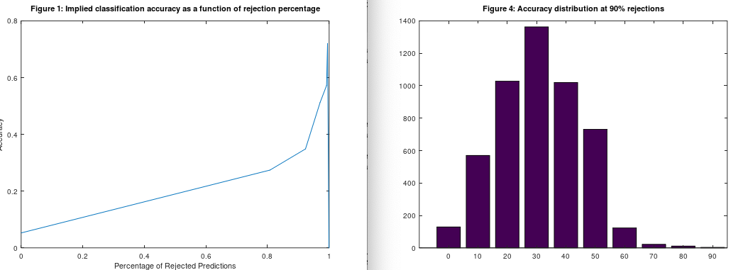
More generally, this implies that the larger a set of random elements is, the less likely it is the elements are independent of each other. To test this empirically, I generated a dataset of 1,000 random vectors, with 1,000 randomly generated classifiers, 1, 2, 3, and 4, and tried to predict the classifier of each vector. I ran Black Tree‘s size-based confidence prediction algorithm on this dataset, which should produce an accuracy of 25%, since these are random vectors, unless something unusual is going on. Unfortunately, this is not included in the free version of Black Tree, but you can do something similar, since it pulls clusters near a given vector and then uses the modal class of the cluster as the predicted class of the given vector. The bigger the cluster, the higher the confidence metric. However, the bigger the cluster, the less likely the vectors in the cluster are to be independent of each other, according to this analysis. And as it turns out, the accuracy actually increases as a function of cluster size, starting out around 27%, and peaking around 70%. The average accuracy for the 90th percentile confidence is about 34%. This makes no sense, in the absence of a theory like the one above. Here’s the code I used to generate the dataset:
Here are the results, with accuracy plotted as a function of confidence, together with the distribution of accuracies at 90% confidence. I ran this algorithm 5,000 times, over 5,000 random subsets of this dataset, and this is the result over all iterations, so it cannot be a fluke outcome. It seems instead the theory is true empirically.
Note that this is not causation. It is instead best thought of as a fact of reality, just like Ramsey’s friends and strangers theorem. Specifically, in this case, it means that information about some of the predictions is almost certainly in their related clusters, because the vectors in the cluster are so unlikely to be independent of one another, despite the fact they were randomly generated. In fact, because they were randomly generated, and not deliberately made to be independent of one another, the more likely outcome is that the vectors are not independent. Therefore, we can use the classifiers of the vectors in the cluster to predict the classifier of the input vector. The larger the cluster, the less likely the vectors are to be mutually independent, resulting in accuracy increasing as a function of cluster size.
As a general matter, if you deliberately cause a set of systems to be totally independent or totally dependent, then those systems are of course not random. If however, you allow the systems to be randomly generated, then the most likely case is that they’re partially dependent upon each other. This is most certainly counterintuitive, but it makes perfect sense, since allowing a random process to control the generation of the systems causes you to lose control of their relationships, and the most likely outcome is that their relationships are dependent upon one another.
I’ve already put the subject of single object classification to bed, however, it dawned on me that there’s an entirely different approach to object classification based upon the properties of the object. We can already say what an object is, that’s not interesting anymore. Instead, what I’m proposing is to describe the object based upon its properties, in particular, texture, which is discernible through image information. Specifically, you have a dictionary of objects, and each object in the dictionary has columns of descriptors such as metallic, matted, shiny, ceramic, and you can of course include color information as well. Then, once an observation has been made, you restrict the cluster returned to those objects that satisfy the observed properties. For example, if the object observed is shiny and ceramic, then less than all objects in the dictionary will be returned. The point is not to say necessarily what the object is, though that would be interesting as well, and instead, to build what is in essence a conceptual model of the object within the machine, beyond a single label.
The applications here are numerous, from unsupervised association between objects based upon visceral information, to potentially new ways to identify objects in a scene based upon small portions of the objects. This latter approach would probably allow you to quickly identify things like leaves, birds, bark, small stones, all of which have unusual textures. Though it would also allow you to make abstract associations between scenes based upon the textures found within them, which could be the seed of real creativity for machines, since it is by definition an abstract association, that is not necessarily dependent upon subject matter or any individual object.
I’m pretty sure I came up with this a long time ago, but I was reminded of it, so I decided to implement it again, and all it does is find edges in a scene. However, it’s a cheap and dirty version of the algorithm I describe here, and the gist is, rather than attempt to optimize the delimiter value that says whether or not an edge is found, you simply calculate the standard deviation of the colors in each row / column (i.e., horizontal and vertical) in the image. If two adjacent regions differ by more than the applicable standard deviation, a marker is placed as a delimiter, indicating part of an edge.
The runtime is insane, about 0.83 seconds running on an iMac, to process a full color image with 3,145,728 RGB pixels. The image on the left is the original image, the image in the center is a super-pixel image generated by the process (the one that is actually analyzed by the delimiter), and the image on the right shows the edges detected by the algorithm. This is obviously fast enough to process real-time information, which would allow for instant shape detection by robots and other machines. Keep in mind this is run on a consumer device, so specialized hardware could conceivably be orders of magnitude faster, which would allow for real-time, full HD video processing. The code is below, and you can simply download the image.
Another one-off, I found a few Andamanese mtDNA genomes in the NIH Database, and the results are consistent with what I’ve read elsewhere, which is that they’re not closely related to Africans, despite being black – turns out being racist is not scientifically meaningful, shocking. However, one interesting twist, it looks like they are closely related to the Iberian Roma and the people of Papua New Guinea. You can find links to the database and the code that will allow you to generate this chart in my paper, A New Model of Computational Genomics.
Astonishingly, they’re monotheistic, and since they’ve been there for about 50,000 years, their religion could be the oldest monotheistic religion in the world, and I’ve never heard anyone even bother to note that they’re monotheistic, which is itself amazing. Moreover, their creation story involves two men and two women, thereby avoiding incest, suggesting they have a better grasp of genetics than Christians – shocking.
I’ve been doing a lot of one-off inquiries in my free time into genetic lineage, and I’m basically always astonished, though this time it’s really something. Specifically, I found this Munda Genome (an ethnic group in India), and it turns out they’re closely related to the Basque and the Swedes, as 50% of the Basque in my dataset and 41% of the Swedes in my dataset are a a 92% match with this genome. You can find links to the dataset and the code to produce this chart in my paper, A New Model of Computational Genomics [1]. The Northern Europeans really do have incredibly interesting maternal lineage, and you can read more about it in [1], as the Finns in particular are truly ancient people, with some of them closely related to Denisovans.


 . Quantize
  so that it creates
  uniform intervals. It follows any sequence of
  predictions can produce any one of
  possible outcomes. Now assume that the predictions generated by
 errors over
 as a constant, and ignore it, we arrive at
  . This is simply the equation for accuracy, multiplied by the number of predictions. However, the number of predictions is relevant, since a small number of predictions doesn’t really tell you much. As a consequence, this is an arguably superior measure of accuracy, that is rooted in information theory. For the same reasons, it captures the intuitive connection between ordinary accuracy and uncertainty.
 to
to  , the state of
  implies the state of lightbulb
  , then you can draw an edge from