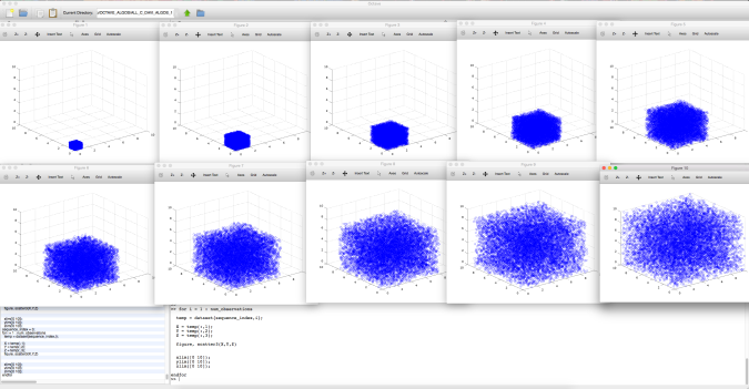
As noted in previous articles, I’ve turned my attention to applying A.I. to thermodynamics, which requires the analysis of enormous datasets of Euclidean vectors. Though arguably not necessary, I generalized a clustering algorithm I’ve been working on to N-dimensions, and it is preposterously efficient:
The attached example takes a dataset of 150,000, 10-dimensional vectors, and clusters them in about 54.2 seconds, with absolutely no errors.
The example is a simple two class dataset, but nonetheless, the efficiency is simply remarkable, and completely eclipses anything I’ve ever heard of, even my own work.
This is particularly useful in thermodynamics, since it lets you cluster points as a function of their distance from an origin, say the center of mass, or the center of some volume. As a result, it allows you to quickly identify the perimeter of a set of points –
Simply take the cluster furthest from the center, which will be last in the list.
So this algorithm is also likely to have applications in object tracking, since you can compress the object to the points at its perimeter, and then track only those points.
This is years into my work, and rather than reexplain things, if you’re interested in how this process works, I’d suggest reading my original paper on machine learning and information theory.
This is another instance of the same ideas in information theory, but in this case, making use of radical compression.
I’m working on the applications of A.I. to thermodynamics, and I had to solve for how to split a dataset into two parts, using objective criteria. Specifically, I’m interested in what’s moving, and what’s not, but the algorithm I came up with is general, and can be used to split any dataset in two, using objective criteria.
It is only a slight tweak on my original clustering algorithm, that requires an additional outer loop that iterates through levels of granularity, because you end up with a coin toss distribution, which produces very slight changes in entropy.
The “final_delta” variable is the threshold value that divides the dataset, so you can test for everything under or over that value, and that’s the dividing line.
The attached code splits a dataset of 50 million real number values in about thirty seconds, running on an iMac.
In previous articles, I introduced my algorithms for analyzing mass-scale datasets, in particular, clustering, and other algorithms. However, those algorithms deliberately avoided operations on the underlying microstate data, since these datasets are comprised of tens of millions of Euclidean vectors.
I’ve now turned my attention to analyzing changes in thermodynamics states, which would benefit from direct measurements of the underlying point data in the microstates themselves. At the same time, any sensible observation of a thermodynamic system is going to consist of at least tens of thousands, and possibly millions of observations. My algorithms can already handle this, but they avoid the underlying point data, and instead use compression as a workaround.
In contrast, the algorithm below actually clusters an enormous number of real value points, with radical efficiency, with the intent being to capture changes in position in individual points in thermodynamic systems.
This is a simple example attached that clusters 225,000 real number values in about 120 seconds, running on an iMac –
This is simply ridiculous.
I’m still refining this algorithm, but thought I would share it now, in the interest of owning claim to it.
The accuracy is just under 100%, though this is a simple example.
You could do this a few times on different dimensions independently, and then take the clusters that each dimension produces in common, using an intersection operator, which is extremely fast in MATLAB.
This will allow you to cluster higher dimensional vectors of numbers, though some vectors might end up not getting clustered using this approach. But with this much data, it probably doesn’t matter.
This would in turn allow you to build a prediction model using any of my prediction algorithms. For my model of prediction, you only need one vector per cluster, and in my admittedly limited experimentation thus far, the number of clusters is quite low, implying that prediction should be fast, despite these enormous datasets.
Attached is software that can generate a graph that represents the transitions of a thermodynamic system, from one state to the next. States that are sequential in time are by definition adjacent, and it’s a directed edge, from the initial state to the next state.
For a thermodynamic system, the underlying state graph is likely to be noise, and mostly disconnected, because microstates could of course occur only once, meaning they have only one next state neighbor.
So in addition, there is code that first clusters the data, into similar states, and then produces a graph based upon items in one cluster transitioning to items in other clusters.
As an example, the attached code uses the expanding gas dataset, over 50 sequences of expansion. So you’d expect the clustering to cause all of the initial states to be clustered together, the later states clustered together, etc, and this is exactly what happens, just as it did in the previous article. As a result, the graph produced should be a path connecting the initial cluster to the final cluster, and this is exactly what happens.
I’ll write some code that allows for visualization of the graphs, but for now, you can examine the matrix to get a sense of its structure:
The graph matrix for the cluster graph
The integer entries indicate how many items the cluster represented by the row is adjacent to. So entry (1,2) shows that cluster 1 is connected to all 50 states in cluster 2, which is exactly what you’d expect, suggesting that the expanding gas always forms a sequence from one state of expansion to the next.
I’ll follow up later this week, possibly today, with software that then uses these graphs to measure how ordered a thermodynamic system is using graph theoretic measures, such as number of maximal paths, how ordered maximal paths are, etc.
NOTE: I corrected a minor bug in a subroutine related to the dictionary insert function, which is updated and attached.
In previous articles, I’ve introduced algorithms that can quickly process datasets that consist of tens of millions of vectors, on a consumer device, allowing for meaningful analysis of the microstates of a thermodynamic system.
In the original article on the topic, I showed how my deep learning algorithms can be used to identify the macrostates of a thermodynamic system, given its microstates.
In a follow up article, I showed how to radically compress a dataset consisting tens of millions of vectors into a dataset of just a few thousand vectors, ultimately using this technique to make radically efficient predictions (about 500 predictions per second, running on an iMac), with perfect accuracy, classifying the rate of expansion of a gas.
In this article, I’ll present a method for measuring how ordered a thermodynamic system is, using a combination of techniques from deep learning and information theory. Specifically, I’ll demonstrate how these techniques can correctly identify the fact that an expanding gas has a progression of states, thereby generating an actual, measurable mathematical order as the gas expands, whereas a stationary gas is essentially unordered, in that any microstate of the gas could in theory appear at any point in time.
Order, Entropy, and Variance
Imagine repeatedly watching the same gas expand, from roughly the same initial volume, to roughly the same final volume, with the number of particles being fixed over each instance of expansion. Further, assume that you took some fixed number of snapshots of the system as it progressed from compressed to expanded, at roughly the same relative moments in time.
Now assume you ran a clustering algorithm on the individual states, as observed. Intuitively, you would expect all of the final, most expanded states to get clustered together, since they are the most similar, structurally. Similarly, you would expect all the initial, compressed states to get clustered together, again, because they are the most similar, structurally.
Now, instead of using typical classifiers, let’s instead put the index at which the state occurs in a hidden dimension. So for example, the first state of an instance of the gas expanding will have a classifier of 1, the second state 2, etc. Since each state of the gas will have a classifier that tells us when it occurred, this will create a distribution of timestamps for each cluster, and if the sequence of observations is truly ordered in terms of timing, then all of the states clustered together should occur at exactly the same timestamp (assuming a relative time stamp, expressed as a length of time since the inception).
So for example, in a truly ordered system, all of the initial states would be clustered together, with no other states; all of the secondary states would be clustered together, with no other states, etc. This is probably not going to work perfectly in the case of a thermodynamic system, since the motions of the particles are highly randomized, but nonetheless, intuitively, you’d expect a stationary gas to be less ordered than an expanding gas, since a stationary gas doesn’t have any noticeable macroscopic change, whereas an expanding gas does, since the volume occupied by the gas is increasing.
We can, therefore, use entropy to measure the consistency of the timestamps within a cluster, since the timestamps will literally generate a distribution. For example, assume that an ideally expanding gas is such that all of its initial states get clustered together, with no other states. The timestamps associated with this cluster would look something like , if we use simple integer timestamps. This distribution will have an entropy of zero, which indicates perfect consistency. In contrast, if a cluster is comprised of similar states that nonetheless occur at totally different points in the sequence, then the entropy will be non-zero.
For these same reasons, we can also use the standard deviation to measure the consistency of the timestamps associated with a cluster. Returning to the example of the ideal gas, the distribution of timestamps will have a standard deviation of zero, whereas a cluster with a diverse set of timestamps will obviously have a non-zero standard deviation.
Together, these two measures allow us to quantify the extent to which a system is ordered, from two different perspectives:
(1) The entropy allows us to measure the multiplicity of outcomes possible;
(2) The standard deviation allows us to measure the variance of when those outcomes occur in time.
Application to Examples in Thermodynamics
As a demonstration, I’ve put together some code attached below that applies these ideas to two datasets:
(A) one is a stationary gas in a fixed volume, represented by 75,000,000 Euclidean three-vectors;
and,
(B) the other is a gas in an expanding volume, also represented by 75,000,000 three-vectors.
The thesis above would imply that the expanding gas is more ordered than the stationary gas, and this is in fact the case.
Beginning with the stationary gas, the first step is to cluster the dataset, using specialized algorithms that I’ve developed to handle enormous datasets of this type –
This takes about 15 minutes, running on an iMac.
Again, rather than attempt to classify the data, we are instead testing for how consistent its positions are in time, so the classifier dimensions are instead integer indexes that tell us at what point in the sequence the state occurred. You could argue that the integers are arbitrary, but this is actually incorrect, and you can use an argument that is similar to the one I use in this article, on the connections between information and error, to show that so long as your observations are always evenly spaced in time, the actual distance in time between observations does not matter for this purpose.
Returning to the measurements described above, we would expect both the entropy and the standard deviation of the expanding gas to be lower than those associated with the stationary gas, and this is in fact the case.
Running the code attached below produced the following measurements:
Stationary Gas:
Average entropy per cluster: 3.9069.
Average standard deviation per cluster: 4.3234.
Expanding Gas:
Average entropy per cluster: 0.87500.
Average standard deviation per cluster: 0.43970.
The command line code is below, and the full archive of my A.I. code is available on ResearchGate.
Following up on the previous article below, attached is an updated command line script that allows for efficient predictions over datasets comprised of tens of millions of observations in Euclidean space.
The specific dataset in the command line code attached models a gas expanding in Euclidean space, at two different rates of expansion, and the prediction task will be to correctly identify the rate of expansion, as either the, “fast one” or the, “slow one”.
Each state of the gas is comprised of 10,000 points in Euclidean space, and each sequence of the gas expanding consists of 15 states, for a total of 150,000 three-dimensional vectors per sequence.
Four frames from one sequence of the gas expanding.
There are 300 sequences, for a total of 45,000,000 three-dimensional vectors.
Obviously, it is, as a general matter, very difficult to analyze datasets that involve this many vectors, but the algorithms I’ve developed can nonetheless quickly and efficiently cluster and then make predictions over datasets of this type, on an ordinary consumer device.
The first step is to sort the data using an operator I introduced in this article, specially designed for mass-scale data –
This first step took about 10 minutes, running on an iMac.
The next step, is to embed each state of the gas on the real number line, using algorithms I introduced in this article –
This step will drastically compress the dataset, from 45,000,000, three-dimensional vectors, to 300, 15-dimensional vectors, with each vector representing a sequence of states of the gas expanding, which took about 25 seconds.
The next step, is to cluster the real-number vectors, which took about .06 seconds.
The final step, is to actually make predictions, which in this case took a total .70 seconds, over the entire dataset of 300 sequences.
The accuracy is in this case perfect with absolutely no errors, given only the first 5 of the 15 observations in each input vector. That is, if you give the prediction algorithm the first 5 states of the gas, it can correctly classify its expansion rate, every time.
My complete set of algorithms is available on ResearchGate, though I’ve also attached the command line code for this particular dataset as a PDF.
This is just the first post in what will be torrent of new algorithms I’ve developed for dealing efficiently with datasets comprised of large numbers of observations.
This set of algorithms implements the dictionary of states referenced in my original article on the topic (the latest article on the topic is here, which links back to the original), allowing for radically efficient comparison between very complex observations, in this case reducing a set of observations to a single dictionary of states.
The net effect of this particular set of algorithms (attached below) is to achieve compression, taking a set of complex observations, that could each consist of thousands of Euclidean datapoints (or significantly more), and quickly eliminate duplicate states, reducing the dataset to a set of unique observations.
The example in the code below takes a sequence of observations intended to model a simple example in thermodynamics, of an expanding gas, which is plotted below.
One sequence from the expanding gas dataset.
Each state of the gas consists of 10,000 points in Euclidean space, and there are 10 observations per sequence, with 10 sequences, for a total of 1,000,000 vectors.
Compression is in this case achieved in about 8 seconds, on an iMac.
This could be useful on its own, but I will follow up with another set of algorithms sometime this week that allow this initial step to facilitate fast prediction over these types of datasets, that consist of massive numbers of observations, even on consumer devices, which would otherwise be intractable, and then follow up with a comprehensive approach to natural language processing using these same algorithms.
The code necessary for this example is available here:
The closing sequence of my book is admittedly weird, and I am plainly suggesting that I’m talking about the mythological figure Sigrid, and not the pop star, and this is deliberate. Though I don’t want to tell people how to think about the text, my read of the facts is that Ida is in fact Sigrid, and if you watch her video, “Strangers”, you’ll see a simply astonishing intersection between the text, and the video –
The plain implication is that Ida’s character is in fact a work of art, from my imagination, and the reveal is that Sigrid is in fact Ida, and that she is a real person. I’ll also note that the full name of the mythological Sigrid is, “Sigrid the Haughty”, which when read aloud, sounds like, “Sigrid the Hottie”, which is not only awesome, and true, but also a Marcel Duchamp reference, to L.H.O.O.Q, which is perfect structurally, since Sigrid appears after the end of the text, like a mustache on the Mona Lisa –
The surprise ending, after the work is already done.
“It starts to rain, and we, we’re the broken beauties”, referencing the flood in the third chapter, as she rises from what looks like a canvas, covered in the shadows of a tree, wearing a yellow shirt, echoing the painting I made for Ida, which has a, “sculptural finish, with a thickness that is significantly raised off the surface of the canvas” (p. 69), as if Sigrid is a painting that’s come to life;
“Blindfolded, minds collide” (00:30), referencing the beers we buy in Sardegna, Ichnusa, the label for which features blindfolded silhouettes, echoing the trope that my true identity has been stolen from me, by bandits;
Ichnusa Beer, featuring four blindfolded silhouettes on the label.
She mirrors the, “Michael Bolton” sequence (p.109), reading a paper, suddenly putting it down (2:24), staring, suggesting a secrete relationship between myself and Sigrid, and of course, she’s angry at the idea that I cheated on her with a Danish celebrity, Mø;
There’s a statue in the video that is plainly a male, stone version of, “Bacchante and Infant Faun”, (00:39) which is referenced in the New York sequence of the text (p. 46);
Bacchante and Infant Faun, by Frederick William MacMonnies (1894).
The drapes hanging are colored like the white marble wall of the bar in Sardegna, which now appears as a soft fabric, that she simply walks through, suggesting visibility into the artistic process (00:48);
The stairs in the background reference the stairs in the studio in Copenhagen, again suggesting you’re now in the studio, getting a glimpse into how things work (01:13);
The giant rocks she’s dancing around (3:13) reference the, “giant sand, or salt crystals” from the artwork in the gallery sequence (p. 187);
Further, the canvas she’s standing in front of (3:37), lit up in green and blue lights, featuring trees, plainly also references the art work that she is likely to have made in the gallery sequence, though almost as if it’s another version, made to represent the beach at night, rather than during the day;
“Memories and photos, too easy to rewrite; left us lonely shadows” (1:27) –
These are simply not normal lyrics for a pop song, especially by someone this young, and it is plainly a subject dealt with explicitly in the text (p. 119).
Sigrid inexplicably, repeatedly screamed like a maniac at a concert, referencing the Eurovision sequence, where a man appears, “basically shouting into a microphone, in what strikes Jeff as most likely to be German”, (p. 117), though Sigrid is obviously a woman, screaming in English;
Watching screens is a repeated theme in the text, as the output of cameras, as a play on observation itself, and the TV plays an inexplicably important role in the aesthetics of rooms, and in substance, providing information that is often critical to a scene, which is clearly referenced in, “Strangers”, and in fact, Sigrid holds a camera, as if watching someone, perhaps me (2:33);
The recording process itself, as a strange invention of modern life, that lets ghosts come back to life (p. 181), also plays a prominent role in the text, and in the video;
The water at the very opening of the video, which has no obvious connection to the rest of the video, references the water while we’re driving after the flood, which represents the power of external objects, like art, to trigger memories, “protecting our memory as well”(p.150);
The words just before each chorus are, “our story’s after the end”, and the final sequence is in fact after the end of the book (p. 214), which actually ends on page 212;
She smiles at the end of the video, alluding to something bordering on funny –
As if she knew that this would all be used in a spectacularly different context, that would inevitably blow someone’s mind (4:02);
Finally, there’s a guy holding a fan (1:05), with my haircut, again suggesting visibility into the artistic process that generated the text –
That you get so see how I did it.
She’s also wearing yellow, in front of a blue backdrop, which is the coloring from our kitchen tiles (p. 125), and the coloring of the sky during the flood (p. 145), and also the color of my scarf in the photo below, demonstrating my artsy do.
Super strange art dude.
The closing sequence would therefore be Ida watching herself on TV, but to resolve this impossibility, given the fact that she, “doesn’t know the song” in question (p. 214), the TV would in this case be playing a song that Ida has not written in this life, or hasn’t written yet, alluding to my ideas on time, which suggest alternate possible realities, and communication between not only different realities, but also from the past into the future, and the future into the past, which is a thread running throughout the entire text, which is in fact itself told almost completely out of order.
This is plainly reflected by the fact that Sigrid has red hair, and green eyes, whereas Ida has blonde hair, and blue eyes, yet I’m saying they are in fact the same person, though there’s a moment in the video for, “Strangers”, where her eyes appear blue in color (2:57), echoing the narrative of the text itself, which is intended to be a sketch, and incomplete in terms of information, with glimpses into what could be interpreted as a memory, but perhaps a memory stored exogenously, by artifacts in the external world, that I’ve strung together, thereby creating an alternate reality, implied by our reality.
Sigrid also says, in the final song referenced in the text, “Dynamite”, “You see, my red is blue”, alluding to subjectivity in perception, despite my belief in an objective reality.
Moreover, the scene of the video for, “Dynamite” is plainly reminiscent of how I described the studio in our home in Copenhagen, with the only objects in sight being a piano and an amplifier (p. 122), in a setting that looks more like a home, than a recording studio. Further, she’s not really wearing much make up, referencing the scene in Carnegie Hall, and appears to be wearing roughly colorless lipgloss (p. 39). The scene also represents the culmination of a path towards freedom for both characters, since we’re both free economically, Ida is free of her trauma, and I’m free of my hatred, if only for the moment –
This places us in a moment that is beyond time and space, where strange things are possible, where location becomes permeable, which is echoed by the opening words to, “Dynamite”, which are, “Don’t know where I am with you; forgetting time and space with you.”
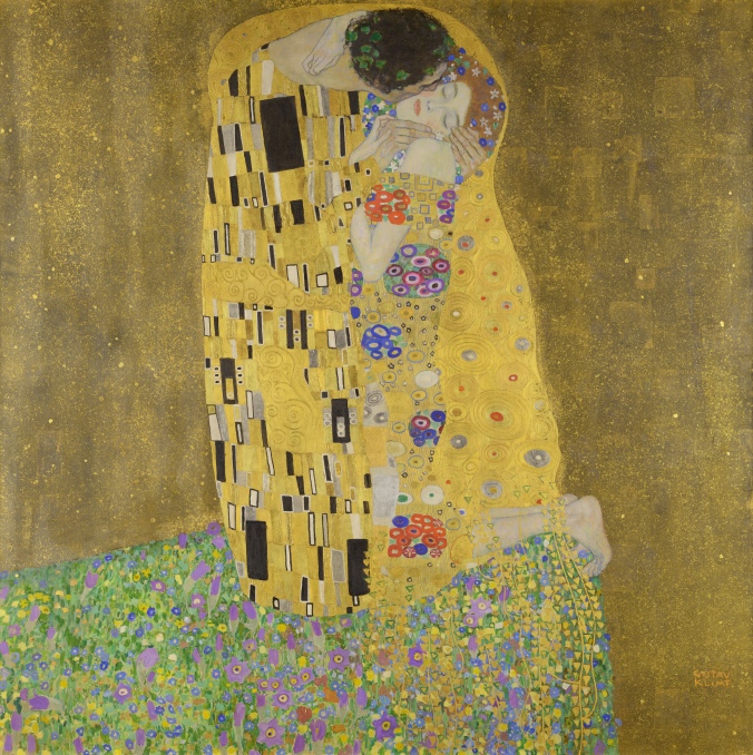
This is also echoed by the closing painting, “The Kiss”, by Klimt, which I’ve rebranded, as “Liebesträume, No. 541”, which in English means, “Love Dream, Number 541”, as if this entire story were just one instance of the relationship between Ida and I –
That we have different names, and different bodies in other outcomes, but nonetheless, the same soul.
The Kiss, by Gustav Klimt (1908).
This is also echoed by the lyrics from Sigrid’s song, “Strangers”, where she says, “Think we got it, but we made up a dream”, and the use of, “Dreams”, by the Cranberries, during the sequence at the beach (p. 85), with the idea being, that if you love someone that much, then moments really do appear surreal, at times, as if you’re dreaming –
That the physical constraints of reality break down, leaving just the two of you, in your own space (p. 5).
This appears again in the sequence in Sardegna, where I look up to find, “a memory mounted into a ceiling” (p. 33), suggesting in the aggregate, that my relationship with Ida is allowing me to recover a, “stolen dream” (p. 33 and 215).
If you buy into the magic, then Sigrid and I somehow created this book together, despite being strangers –
That what I said about our relationship is physically true, in that Ida and I, “contribute to a moving portrait, that we share, together, as coauthors and spectators of an uncertain future, and a certain now.” (p. 105), perhaps so we could rediscover each other.
Finally, I’ll note that my plainly bespoke and artsy hairdo inexplicably appears at 1:05 in Sigrid’s video for, “Strangers”, the quote suggesting we wrote the work together appears on page 105 of my book, and “EDA” backwards is “ADE”, which when expressed in numerals is, “145”, and from a distance, it’s not unreasonable to confuse a, “4” with a, “0”, but like I say in the book, it seems as though we all have, “eye problems” (p. 198).
Attached is an updated version of my book, “Sketches of the Inchoate”, which now includes an additional set of songs that accompany the text, meant to convey Ida’s state of mind throughout the story.
I’ve put together an admittedly experimental form-of-art playlist to accompany my book, “Sketches of the Inchoate”, comprised of six songs, to echo the six chapters of the book.
I’m not going to provide any heavy analysis on the meaning, and instead, deliberately float it, allowing for ambiguity and interpretation, unlike the actual accompanying music, which has a fairly clear meaning in each scene, that I’ve generally worked through.
The overall sequence of this playlist is intended to operate as a metaphor for Ida’s character, transitioning from having a secret, confronting trauma, twice, and then ultimately transitioning to motherhood, and grace –
The moments when she stares out of windows, singing to herself, the idea being that the future communicates with the present, and so Ida can hear her future children singing to her, at times, pulling her towards the realization of motherhood.

 , if we use simple integer timestamps. This distribution will have an entropy of zero, which indicates perfect consistency. In contrast, if a cluster is comprised of similar states that nonetheless occur at totally different points in the sequence, then the entropy will be non-zero.