Note on the Riemann Zeta Function

As you know, I’ve been doing research in information theory, and some of my recent work has some superficial connections to the Zeta function, since I was making use of logarithms of complex numbers.

I noticed the following graph:

ReZero-n6


In short, we’d be looking at the Zeta function using values of s produced by powers of the logarithm function:

zeta(log^n (-1) /x).

There appears to be several zeros for n = 6.

You can see it yourself on wolfram using the following link:

But, I don’t know enough about this topic to be sure that this is actually interesting, since I know that at least some of the zeros of this function are considered “trivial”.

Nonetheless, I thought I’d share this in case some of you found it interesting and had insights.

Regards,

Charles

On the Applications of Information Theory to Physics

I’ve attached an updated draft of what is in effect a summary of the work I’ve been doing applying information theory to physics, that I thought some of you would find interesting, given the popularity of my work on the connections between information theory and artificial intelligence.

Despite the imposing title, the attached note is actually a straightforward explainer that a computer scientist or mathematician with almost no background in physics will have no trouble understanding. In fact, it arguably doubles as a quick explainer on what are in my opinion some very interesting issues in physics.

The full suite of related articles is available on my researchgate homepage here.

Happy Holidays,

Charles

Non-Local Interactions, Spin, the Strong and Weak Forces, Inertia, and Faraday Induction (1) (1)

Fast N-Dimensional Categorization Algorithm

In a previous post entitled, “Using Information Theory to Create Categories with No Prior Information”, I presented an algorithm that can quickly construct categories given a linear dataset with no other prior information. In this post, I’ll present a generalization of that algorithm that can be applied to a dataset of n-dimensional vectors, again with no prior information. Like all of the other work I’ve presented as part of this project, this algorithm is again rooted in information theory and computer theory. For an explanation as to why this algorithm works, you should see the post below, as this is really just a generalization of the previous algorithm applied to higher dimensional data, with no meaningfully new theory.

In this post, I’m going to focus on the results of this algorithm, which are quite good. I’ll also discuss the runtime complexity of the algorithm, which I believe to be worst-case O(log(n)n^{D+1}), where D is the dimension of the dataset, making this algorithm exceptionally fast for what it is, which is a data categorization algorithm.

As a general matter, the only thing that this algorithm requires is a dataset that has a measure function that maps to a real number. In simpler terms, all we need in order to make use of this algorithm is a function that can compare the “distance” between any two data points in the dataset. This means that we can apply this algorithm to any n-dimensional dataset simply by making use of the norm of the difference between any two vectors in the dataset, and that we can also apply this algorithm to non-Euclidean spaces, so long as we have a well-defined measure function on the space.

In a follow up post, I’ll show how we can actually use this algorithm to produce a well-defined measure in classification problems by iterating through different measures until we produce the “right” measure that results in the maximum change in the structure of our classification.

Runtime Complexity

The first thing that this algorithm does is test the symmetry of the dataset using a function called “partition_array”, which is attached together with all of the other scripts you need to run this algorithm. Partition_array repeatedly subdivides the space in which the dataset exists into smaller and smaller “chunks”, until each chunk contains a maximally different amount of information. In this case, just imagine breaking a cube of 3-space into smaller and smaller equally sized subcubes. As we do this, the number of data points within each subcube will vary as a function of the number of subdivisions, with the number of data points per subcube generally decreasing as a function of the number of subdivisions, simply because each subcube will get smaller as we increase the number of subdivisions.

For reasons explained below, this algorithm stops once it finds the partition size that maximizes the standard deviation of the information contained within each subcube. This will produce a number N, which is how many times we’ve subdivided each dimension in order to achieve this maximization. It turns out that N is a measure of how symmetrically the data is distributed within its own space. If N is large, then the data is symmetrically distributed. If N is small, then the data is asymmetrically distributed.

The partition_array algorithm begins by making an initial guess as to the value of N, which it sets to the log of the number of the items in the dataset. Then, depending upon the characteristics of the dataset, it will either increase its guess, or decrease its guess, by either multiplying its first guess by 2, or dividing its first guess by 2, respectively. It will continue doing this until it finds the value of N that maximizes the standard deviation of the information contained in each subcube, which will cause the value of N to increase, or decrease, exponentially. However, the algorithm prevents N from increasing past the number of items in the dataset, and also prevents it from decreasing below 1. As a result, if n is the number of items in the dataset, then the partition_array algorithm runtime complexity cannot exceed log(n).

For each value of N generated by partition_array, another function called “test_entropy” is called. This is the function that actually tests the information content of each subcube. As part of this function, we will have to test each item in the dataset to determine which subcube it belongs to. Because we divide each dimension N times, which generates N^3 subcubes, and N is necessarily less than or equal to n, it follows that the number of subcubes cannot exceed n^3. As a result, we’ll have to do at most n^4 comparisons each time we call test_entropy.

As a general matter, this implies that the runtime complexity of this phase of the algorithm is necessarily less than,

log(n)n^{D+1},

where D is the dimension of the space. In this case, D = 3, and therefore, the worst-case runtime complexity is log(n)n^4.

Though this is only the preprocessing phase of the algorithm, it is actually the part of the algorithm with the highest worst-case runtime complexity. As a result, this algorithm has an overall worst-case runtime complexity of O(log(n)n^{D+1}), making it extremely fast for what it does.

In a follow up post, I’ll present a vectorized categorization algorithm that omits this step, allowing for extremely fast categorization of high-dimensional data.

Anecdotally, I’ve noticed that the algorithm makes short work of data that actually has structure, and struggles with data that is truly randomized. This is not surprising, since truly randomized data should be highly symmetrical, forcing the preprocessing stage into the worst-case runtime (i.e., producing a very large value of N).

Application to Data

I’ve attached a set of scripts that make it easy to test the algorithm, which should be called from the Octave command line as follows:

pkg load image

pkg load communications

data_array = generate_n_random_categories_3D(base, adjustment, min_spread, max_spread, num_items, num_categories);

data_categories_array = optimize_categories_3D(data_array);

[X Y Z S C] = display_categorization_3D(data_categories_array,num_items);

figure, scatter3(X,Y,Z,S,C);

The generate_n_random_categories_3D script does exactly what its name suggests, which is to generate categories of random vectors in 3-space. The script creates what we know to be categories of data by randomly generating a set of seed values, around which it will generate some random data points.

So, for example, if num_categories = 2, and num_items = 1000, then it will create 2 categories of data that each contain 500 data points. This is accomplished by generating 2 seed locations, about which each category is centered. These seed locations can be anywhere from [0 0 0] to [base base base]. As a result, the greater the value of base is, the greater the space in which the data exists. Therefore, a small number of categories and a large value of base increases the probability that our categories will be very far apart.

The min_spread and max_spread control how diffuse the data is around each category’s central point. The first category generated has the minimum diffusion, and the last category generated has the maximum diffusion, with diffusion increasing linearly with each category generated. A high value of adjustment in essence forces each category’s central point to be generated along the same line, and a zero value of adjustment allows the central points to be generated randomly throughout the entire space from [0 0 0] to [base base base].

The “optimize_categories_3D” algorithm takes the data, and sorts it into categories, using the process I described above, which are then formatted for display by the “display_categorization_3D” function.

Data points are represented by the little ‘o’ rings in the attached images. When two data points are part of the same category, the display algorithm paints them with the same color. However, because category colors are randomly generated, it’s possible for two different categories of data to be assigned approximately the same color, and, though extremely unlikely, it’s even possible they’re assigned the exact same color. As a result, local colors are what to look for if you want to determine what data points are part of the same category.

The size of the ring representing a data point is determined by the size of the category to which the data point belongs. If the data point is part of a big category, then the ring will be big. If the data point is part of a small category, then the ring will be small.

I’ve attached graphs from two series of datasets, one for which the value of adjustment is high, forcing categories to be generated along a roughly straight line, and another for which the value of adjustment is zero, allowing categories of data to be spontaneously generated anywhere within the space bounded by [0 0 0] to [base base base].

The first series consists of 11 datasets, with all of the inputs to the random data generator remaining constant for each data set, except the value of max_spread, which increases from the first dataset to the last dataset. Each dataset in the first series consists of 50 categories, with 10 points in each category, for a total of 500 data points per data set. The first dataset in this series looks like a series of tightly packed rings, since for the first dataset, the min_spread equals the max_spread, meaning that each of the categories in this dataset should be roughly identically distributed, and just seeded at different locations in the space. As we move through this series of datasets, max_spread increases, meaning that the first category in each dataset will be more tightly packed than the last category in that same data set. This is why the last dataset in this series looks like a lot like a confetti cannon, since the first category in that data set is tightly packed, and the last category is extremely diffuse, representing the maximum possible spread for that entire data set.

Looking at the results, you can clearly see that the algorithm generates intuitively correct categorizations, grouping tightly packed clusters into a small number of relatively large categories, and diffuse clusters into a large number of relatively small categories. The last two charts show how many categories the algorithm actually generates for each series. Specifically, as max_spread increases, the number of categories generated for each of the 11 datasets in this series is as follows:

46 42 46 66 73 78 88 86 106 85 126

Note that 50 categories is in some sense the “correct” answer, since that is the number of clusters generated by the underlying random data generator. However, as the diffusion of each cluster increases, the clusters will become more diffuse, causing each cluster to lose its structure, and causing neighboring clusters to overlap. As a result, we should expect the number of categories identified by the algorithm to increase as a function of diffusion, which is exactly what happens.

chart

The next series of datasets is generated using exactly the same variables, except the value of adjustment is set to 0, and the difference between the min and max spread is smaller to account for the smaller space the data occupies (this is a consequence of adjustment being set to 0). As a result, in this case, the seed values for the clusters propagate randomly throughout the entire space. This causes the datasets to start out in little tightly packed clusters that are randomly distributed, and eventually diffuse into generally unstructured data with a few small local clusters that the algorithm does a great job of categorizing together, when appropriate.

As max_spread increases, the number of categories generated for each of the 11 data sets is as follows:

46 180 265 321 261 297 331 329 365 375 246

Again, 50 is arguably the “correct” answer. However, in this case, the algorithm is clearly far more sensitive to diffusion in the data, which isn’t surprising, since in this case, we haven’t constrained the diffusion at all, but instead, have allowed the data to propagate randomly throughout the entire space.

chart

To generate the “confetti cannon” data, use the following:

base = 10;
adjustment = 50;
min_spread = 1;
num_items = 500;
num_categories = 50;

for i = 0 : 10

max_spread = 1 + 15*i;
data_array = generate_n_random_categories_3D(base, adjustment, min_spread, max_spread, num_items, num_categories);
data_categories_array = optimize_categories_3D(data_array);
[X Y Z S C] = display_categorization_3D(data_categories_array,num_items);
figure, scatter3(X,Y,Z,S,C)

endfor

To generate the randomly clustered data, use the following:

base = 25;
adjustment = 0;
min_spread = .1;
num_items = 500;
num_clusters = 50;

for i = 0 : 10

clear data_categories_array
max_spread = .1 + .45*i;
data_array = generate_n_random_categories_3D(base,adjustment, min_spread, max_spread, num_items, num_clusters);
tic; data_categories_array = optimize_categories_3D(data_array);toc
[X Y Z S C] = display_categorization_3D(data_categories_array, 500);
figure, scatter3(X,Y,Z,S,C)

endfor

In a follow up post, I’ll show how we can categorize new data, and predict to which category new data fits best, using the opposite approach: that is, we find the dataset of best-fit for new data by including the new data into a series of datasets, and the dataset that changes the least in terms of the structure of its categories is the dataset to which the new data fits best. We measure the change in structure of the categories by using the entropy of the categorization, just as we did above. In short, new data fits best where it disturbs category structure the least, and we measure change in category structure using the entropy of the categorization.

The relevant Octave scripts are available here:

display_categorization_3D

find_most_distant_pair

generate_categories_3D

generate_n_random_categories_3D

left_right_delta_3D

optimize_categories_3D

partition_array_3D

test_entropy_array_3D

A Simple Model of Non-Turing Equivalent Computation

Alan Turing’s statement of what is now known as the Church-Turing Thesis asserts that all forms of “mechanical” computation are equivalent to a Universal Turing Machine. The Church-Turing Thesis is not a mathematical theorem, but is instead a hypothesis that has turned out to be true as an empirical matter. That is, every model of computation that has ever been proposed has been proven to be capable of computations that are either equivalent to, or a subset of, the computations that can be performed by a UTM.
 
Nonetheless, as I’ve discussed in previous posts, there are good reasons to believe that nature itself is capable of generating non-computable processes. First off, it is mathematically impossible for a UTM to generate information (see the post below for a simple proof). Nonetheless, human beings do this all the time. In fact, I’m doing exactly that right now.
 
At the same time, Alan Turing is one of my personal heroes, so it’s not easy for me to disagree with him. He’s also a cosmically intelligent human being that I don’t disagree with, without extreme caution. As a result, I’ll hedge my bets and say that what I present below is exactly what he was hoping to be true: that there is a simple model of computation beyond the UTM, and that nature is, as common sense suggests, stranger and more complicated than even the strangest fiction.
 
The “Box”
 
We naturally associate computation with symbolic computation, since that’s what we’re taught to do from the time we’re born. That is, computation is what you to do numbers and symbols, and computers are tools you use to do a lot of computations in a short amount of time. This view is embedded in the Church-Turing Thesis itself, in that Turing described computation as an inherently “mechanical” process. But when you compress the input to a UTM maximally, what you really have is a “trigger”. That is, there’s some string that we provide as the input to some box, and then that box spontaneously generates some output. That input string will probably be totally unrecognizable as anything that should be associated with the output that it will ultimately generate, since, by definition, we’ve eliminated all the compressible structure in the input, leaving what will be a maximally randomized kernel.
 
Abstracting from this, we can define a kind of computation that is not the product of mathematical operations performed on a set of symbols. Instead, we can view the input to a computational device as a trigger for the outputs that follow. This view allows us to break free of the mathematical restraints of mechanical computation, which prevent us from generating complexity. That is, as noted above, and proven below, the complexity of the output of a UTM can never exceed the complexity of its input. If, however, we treat the input to a device as a trigger, and not the subject of some mathematical operation, then we can map a finite string to anything we’d like, including, for example, a particular configuration of a continuous surface.
 
Implementing this would require a continuous system that responds to inputs. Some kind of wave seems to be the best candidate, but I’m not claiming to know what physical systems we should use. Instead, I’m presenting what I believe to be a simple mathematical model of computation that is on its face non-computable, and leaving it up to the adults in the room to figure out how to implement it.
 
Assume that we have some input m, that we give to our computational device X.
In particular, let’s assume X is always in some state that we’ll represent as a series of integer values mapped to an uncountable space. That is, the state of X can be represented as an uncountable multi-set of integers, which for convenience we’ll imagine being represented as heights in a plane. Specifically, imagine an otherwise flat plane that has some height to it, with the height of the plane at a given point representing the value of the state of X at that point, and the aggregate set of heights representing the overall state of X at a given moment in time.
 
When X is given some input m, assume that its state changes from some X_0, to some other state X(m).
 
We could assume that the state of X changes for some period of time after receiving the input m, or switches immediately to X(m). Either way, the important part is to assume that X is, by definition, capable of being in states that require an infinite amount of information to fully represent. We could of course also allow X to be in states that require only a finite amount of information to represent, but the bit that will make X decidedly non-computable is the ability to be in a state that is in effect a chaotic wave. That is, a discontinuous set of integer values mapped onto a continuous surface, that, as a result, cannot be compressed into some finite representation.
 
If such a system exists, X would be, by its nature, non-computable, since, first of all, X generates states that require an uncountable number of integers to fully represent. Since a UTM can generate only finite outputs, the states of X cannot be simulated by a UTM. Further, X is capable of being in non-compressible, infinitely complex states, which means that there is no finite compression of at least some of the states of X, again implying that, even if we could “read” every point on the surface of X, there are at least some states of X that could not be compressed into a finite string that could in turn generate the complete state of X on some UTM.
 
As a result, if such a system exists, then we would be able to take a finite string, and trigger an output that contains an infinite amount of information, generating complexity. Further, by juxtaposing two waves directly on top of each other, we would presumably generate constructive interference, the result of which we could define as the “sum” of two inputs. By juxtaposing two slightly offset waves, we would presumably generate destructive interference, the result of which we could define as the “difference” between two inputs. As a result, if we could understand and control such a system, perhaps we could perform otherwise non-computable computations.

Correlation, Computability, and the Complexity of Music

If we know truly nothing at all about a data set, then the fact that the data is presented to us as a collection of vectors does not necessarily imply that there is any connection between the underlying dimensions of the vectors. That is, it could just be a coincidence that has caused these otherwise independent dimensions of data to be combined into vector form. This suggests that whether we create categories based upon the vectors as a whole, or the individual dimensions of the vectors, will depend upon our ex ante assumptions about the data.

Even in the case where the components of the vectors are not statistically correlated, it could still nonetheless be rational to treat the components as part of a whole. This would be the case whenever a combination of underlying characteristics affects the whole. Color is a good example of this. As a general matter, we’ll probably want to categorize colors as a whole (i.e., a single RGB vector), but the individual components of a data set of colors might not necessarily be correlated with each other. That is, we could be given a data set of colors where the red, blue, and green luminosity levels are all statistically independent of each other. Nonetheless, the combinations of color luminosities determine the perceived colors, and therefore, we can rationally construct categories using entire vectors, and not just the components of the vectors, despite the fact that the components of the vectors might be statistically independent of each other. In this case, this is driven by a perceptual phenomenon, since it just happens to be the case that the brain combines different exogenous wavelengths of light into a single perceived color.

This example highlights the distinction between (1) statistical correlation between the components of a vector, and (2) the co-relevance of the components of a vector in their contribution to some whole that is distinct from its underlying components.

Similar ideas apply to music, where a chord produces something that is distinct from its individual components. That is, when a single note is played, there is no harmony, since by definition there is only one note. This is in some sense a point of semantics, but it can also be expressed mathematically. That is, when a single note is played, there is no relationship to be considered between any two notes, since there is, of course, only one note. When two notes are played, however, not only are there two auditory signals being generated, but there is a third distinct artifact of this arrangement, which is the relationship between the two notes. As we add notes to the chord, the number of relationships between the notes increases.

We can count these relationships using simple combinatorics. For example, 3 notes played simultaneously creates 7 distinct perceptual artifacts. Specifically, there are the 3 individual notes; the 3 combinations of any two notes; and the 1 combination of all 3 notes. An untrained musician might not be conscious of these relationships, whereas a trained musician will be. But in either case, in a manner more or less analogous to how a blue and a red source produce magenta, which is a non-spectral color, two or more notes generate higher order perceptual experiences that are fundamentally different than those generated by their individual components. That is, harmony is a perceptual experience that must be distinct from the signals generated by its underlying components, since certain combinations of notes are known to be harmonious, whereas others are not, and instead produce dissonance (i.e., combinations of notes that “clash”).

Unlike visual art, which exists in a Euclidean space, music extends through time, in a fairly rigorous manner, with definite mathematical relationships between the notes played at a given moment, and between the notes played over time. Moreover, these relationships change in a non-linear manner as a function of the underlying variables. For example, a “major third” is arguably the most pleasant sound in music, and is generally associated with an expression of joy (think of the melody from Beethoven’s, “Ode to Joy”). One half-step down (which is the minimum decrement in the 12-tone scale), and we find the minor third, which, while harmonious, is generally associated with an expression of sadness (think of the opening to Beethoven’s, “Moonlight Sonata”). One whole-step down from a major third, we find a harmonically neutral combination between the root of a chord and the second note in the related scale. That is, adding this note to a chord doesn’t really change the character of the chord, but adds a bit of richness to it. In contrast, one whole step up from a major third, and we find a tritone, which is a dissonance so visceral, it’s generally associated with evil in cheesy horror movies, producing a demented sound (have a listen to the opening of “Totentanz”, by Franz Liszt).

In short, though there are undoubtedly patterns in music, the underlying space is extremely complex, and varies in an almost chaotic manner (at least over small intervals) as a function of its fundamental components.

This suggests that generating high-quality, complex music is probably a much harder problem than generating high-quality visual art. With all due respect to visual artists, the fact is that you can add statistical noise to the positions of pixels in a Picasso, and it will still look similar to the original piece. Similarly, you can add statistical noise to its colors, and nonetheless produce something that looks close to the original piece. As a result, it suggests that you can “approximate” visual art using statistical techniques. This is a consequence of the space in which visual art exists, which is a Euclidean physical space, and a roughly logarithmic color space. In contrast, if you “blur” Mahler’s 5th Symphony, changing the notes slightly, you’re going to produce a total disaster. This is a consequence of the underlying space in music, which is arguably chaotic over small intervals, though it certainly has patterns over large intervals.

Upon reflection, it is, therefore, actually remarkable that human beings can take something as complex as a symphony, which will have an enormous number of relationships to consider, that change randomly as a function of their underlying variables, and reduce it to a perceptual experience that is either harmonious or not. The ability to create something so complex that is nonetheless structured, and perceived in a unitary manner by others, borders on the astonishing.

It suggests that the minds of people like Mozart, Beethoven, and Brahms, could provide insights into how some human beings somehow operate as net contributors of structured information, despite the fact that it is mathematically impossible for a classical computer to generate “new information”, since the Kolmogorov complexity of the output of a Turning Machine is always less than or equal to the complexity of its input. That is, a Turing Machine can alter, and destroy information, but it cannot create new information that did not exist beforehand.

This can be easily proven as follows:

Let K(x) denote the computational complexity of the string x, and let y = U(x) denote the output of a UTM when given x as input. Because x generated y, by definition, K(y) \leq |x|. Put informally, K(y) is the length, measured in bits, of the shortest program that generates y on a UTM. Since x generates y when x is given as the input to a UTM, it follows that K(y) can’t be bigger than the length of x. This in turn implies that K(y) \leq K(x) + C. That is, we can generate y by first running the shortest program that will generate x, which has a length of K(x), and then feed x back into the UTM, which will in turn generate y. This is simply a UTM that “runs twice”, the code for which will have a length of C that does not depend upon x, which proves the result. That is, there’s a UTM that always runs twice, and the code for that machine is independent of the particular x under consideration.

We could, therefore, take the view that meaningful non-determinism is the best evidence for computation beyond what is possible by a UTM.

That is, if a source generates outputs, the complexities of which consistently exceed the aggregate complexities of any apparent inputs, then that source simply cannot be computable, since, as we just proved above, computable processes cannot generate complexity. If it is also the case that this source generates outputs that have structure, then we cannot say that this source is simply producing random outputs. Therefore, any such source would be a net contributor of structured information, which means that the source would be a non-random, non-computable source.

I am clearly suggesting the possibility that at least some human beings are capable of producing artifacts, the complexities of which exceed the aggregate complexities of any obvious sources of information. In short, human creativity might be the best evidence for non-random, non-computable processes of nature, which would in turn, imply that at least some human beings are fundamentally different from all known machines. This view suggests that, similarly, our greatest mathematicians weren’t operating as theorem provers, beginning with assumptions and mechanistically deducing conclusions, but were perhaps arriving at conclusions that did not follow from any obvious available sources of information, with minds that made use of processes of nature that we do not yet fully understand. This is probably why these people are referred to as geniuses. That is, the artifacts produced by people like Newton, Gauss, and Beethoven are astonishing precisely because they don’t follow from any obvious set of assumptions, but are instead only apparent after they’ve already been articulated.

But in addition to the admittedly anecdotal narrative above, there is also a measure of probability developed by Ray Solomonoff that provides a more convincing theoretical justification for the view that human creativity probably isn’t the product of a computable process. Specifically, Solomonoff showed that if we provide random inputs to a UTM (e.g., a binary coin toss), then the probability of that UTM generating a given output string x is given by,

p \approx 1/2^{K(x)},

where K(x) is the same Kolmogorov complexity of x we just discussed above. That is, the probability that a UTM given random inputs generates a given string x is approximately equal to 1/2^{K(x)}.

We can certainly iteratively generate all binary inputs to a UTM, and it is almost certainly the case that, for example, no one has stumbled upon the correct input to a UTM that will generate Mahler’s 5th symphony. So, if we want to argue that the creative process is nonetheless the product of a computable process, it follows that the computable process, in this case, Mahler’s creative process, is the product happenstance, where a series of random inputs serendipitously found their way to Gustav Mahler, ultimately causing his internal mental process to generate a masterpiece.

In addition to sounding ridiculous when stated in these terms, it turns out that Solomonoff’s equation above also casts serious doubt on this as a credible possibility. Specifically, because we’ve presumably yet to find the correct input to a UTM that will generate Mahler’s 5th symphony, this input string is presumably fairly large. This implies that the probability that an encoded version of Mahler’s 5th will be generated by a UTM given random inputs is extremely low. As a result, we’re left with the conclusion that large, high-complexity artifacts that nonetheless have structure are probably not the product of a random input being fed to a UTM. Moreover, such artifacts are even less likely to be the product of pure chance, since K(x) \leq |x| + C. That is, we can just feed the input x to a UTM that simply copies its input, so a string is never more complex than its own length plus a constant. As a result, assuming x is an encoding of Mahler’s 5th symphony, we’re probably far more likely to randomly generate y, for which U(y) = x, than we are to generate x itself. But as we just showed above, both of these outcomes have probabilities so small that it’s probably more sensible to assume that we just don’t understand how some people think.

As a result, Solomonoff’s equation expresses something we all know to be true in mathematical terms: I can toss coins for a billion years, and I’ll still never produce something like Mahler’s 5th. In the jargon of computer theory, Mahler’s 5th Symphony might be the best evidence that the Church-Turing Thesis is false.

This view is even more alarming when you consider the algorithmic probability of generating a DNA molecule…

Using Information Theory to Create Categories with No Prior Information

In a previous post below entitled, “Image Recognition with No Prior Information”, I introduced an algorithm that can identify structure in random images with no prior information by making use of assumptions rooted in information theory. As part of that algorithm, I showed how we can use the Shannon entropy of a matrix to create meaningful, objective categorizations ex ante, without any prior information about the data we’re categorizing. In this post, I’ll present a generalized algorithm that can take in an arbitrary data set, and quickly construct meaningful, intuitively correct partitions of the data set, again with no prior information.

Though I am still conducting research on the run-time of the algorithm, the algorithm generally takes only a few seconds to run on an ordinary commercial laptop, and I believe the worst case complexity of the algorithm to be O(log(n)n^2 + n^2 + n), where n is the number of data points in the data set.

The Distribution of Information

Consider the vector of integers  x = [1 2 3 5 10 11 15 21]. In order to store, convey, or operate on x, we’d have to represent x in some form, and as a result, by its nature, x has some intrinsic information content. In this case, x consists of a series of 8 integers, all less than 2^5 = 32, so we could, for example, represent the entire vector as a series of 8, 5-bit binary numbers, using a total of 40 bits. This would be a reasonable measure of the amount of information required to store or communicate x. But for purposes of this algorithm, we’re not really interested in how much information is required to store or communicate a data set. Instead, we’re actually more interested in the information content of certain partitions of the data set.

Specifically, we begin by partitioning x into equal intervals of Δ = (21-1) / N, where N is some integer. That is, we take the max and min elements, take their difference, and divide by some integer N, which will result in some rational number that we’ll use as an interval with which we’ll partition x. If we let N = 2, then Δ = 10, and our partition is given by {1 2 3 5 10 11} {15 21}. That is, we begin with the minimum element of the set, add Δ, and all elements less than or equal to that minimum + Δ are included in the first subset. In this case, this would group all elements from 1 to 1 + Δ = 11. The next subset is in this case generated by taking all numbers greater than 11, up to and including 1 + 2Δ = 21. If instead we let N = 3, then Δ = 6 + ⅔, and our partition is in this case given by {1 2 3 5} {10 11} {15 21}.

As expected, by increasing N, we decrease Δ, thereby generating a partition that consists of a larger number of smaller subsets. As a result, the information content of our partition changes as a function of N, and eventually, our partition will consist entirely of single element sets that contain an equal amount of information (and possibly, some empty subsets). Somewhere along the way from N = 1 to that maximum, we’ll reach a point where the subsets contain maximally different amounts of information, which we treat as an objective point of interest, since it is an a priori partition that generates maximally different subsets, at least with respect to their information content.

First, we’ll need to define our measure of information content. For this purpose, we assume that the information content of a subset is given by the Shannon information,

I = log(1/p),

where p is the probability of the subset. In this case, the partition is a static artifact, and as a result, the subsets don’t have real probabilities. Nonetheless, each partition is by definition comprised of some number of m elements, where m is some portion of the total number of elements M. For example, in this case, M = 8, and for Δ = 6 + ⅔, the first subset of the partition consists of m = 4 elements. As a result, we could assume that p = m/M = ½, producing an information content of log(2) = 1 bit.

As noted above, as we iterate through values of N, the information contents of the subsets will change. For any fixed value of N, we can measure the standard deviation of the information contents of the subsets generated by the partition. There will be some value of N for which this standard deviation is maximized. This is the value of N that will generate maximally different subsets of x that are all nonetheless bounded by the same interval Δ.

This is not, however, where the algorithm ends. Instead, it is just a pre-processing step we’ll use to measure how symmetrical the data is. Specifically, if the data is highly asymmetrical, then a low value of N will result in a partition that consists of subsets with different numbers of elements, and therefore, different measures of information content. In contrast, if the data is highly symmetrical, then it will require several subdivisions until the data is broken into unequally sized subsets.

For example, consider the set {1, 2, 3, 4, 15}. If N = 2, then Δ = 7, and immediately, the set set is broken into subsets of {1, 2, 3, 4} and {15}, which are of significantly different sizes when compared to the size of the original set. In contrast, given the set {1, 2, 3, 4, 5}, if N = 2, then Δ = 2, resulting in subsets of {1, 2, 3} {4, 5}. It turns out that the standard deviation is in this case maximized when N = 3, resulting in a partition given by {1, 2} {3} {4, 5}. We can then express the standard deviation of the partition as an Octave vector:

std( [ log(5/2) log(5) log(5/2) ] ) = 0.57735.

As a result, we can use N as a measure of symmetry, which will in turn inform how we ultimately group elements together into categories. The attached partition_vec script finds the optimum value of N.

Symmetry, Dispersion, and Expected Category Sizes

To begin, recall that N can be used as a measure of the symmetry of a data set. Specifically, returning to our example x = [1 2 3 5 10 11 15 21] above, it turns out that N = 2, producing a maximum standard deviation of 1.1207 bits. This means that it requires very little subdivision to cause x to be partitioned into equally bounded subsets that contain maximally different amounts of information. This suggests that there’s a decent chance that we can meaningfully partition x into categories that are “big” relative to its total size. Superficially, this seems reasonable, since, for example, {1 2 3 5} {10 11 15} {21} would certainly be a reasonable partition.

As a general matter, we assume that a high value of N creates an ex ante expectation of small categories, and that a low value of N creates an ex ante expectation of large categories. As a result, a high value of N should correspond to a small initial guess as to how different two elements need to be in order to be categorized separately, and a low value of N should correspond to a large initial guess for this value.

It turns out that the following equation, which I developed in the context of recognizing structure in images, works quite well:

divisor = N^{N(1-symm)}/ 10,

where divisor is the number by which we’ll divide the standard deviation of our data set, generating our initial minimum “guess” as to what constitutes a sufficient difference between elements in order to cause them to be categorized separately. That is, our initial sufficient difference will be proportional to s / divisor.

“Symm” is, as the name suggests, yet another a measure of symmetry, and a measure of dispersion about the median of a data set. Symm also forms the basis of a very simple measure of correlation that I’ll discuss in a follow up post. Specifically, symm is given by the square root of the average of the sum of the squares of the differences between the maximum and minimum elements of a set, the second largest and second smallest element of a set, and so on.

For example, in the case of the vector x, symm is given by,

[\frac{1}{8} ( (21 - 1)^2 + (15 - 2)^2 + (11 -3)^2 + (10 - 5)^2 + (10 - 5)^2 + (11 -3)^2 + (15 - 2)^2 + (21 - 1)^2 )]^{\frac{1}{2}},

which is 12.826.

As we increase the distance between the elements from the median of a data set, we increase symm. As we decrease this distance, we decrease symm. For example, symm([ 2 3 4 5 6 ]) is greater than symm([ 3 3.5 4 4.5 5 ]). Also note that a data set that is “tightly packed” on one side of its median and diffuse on the other will have a lower value of symm than another data set that is diffuse on both sides of its median. For example, symm([ 1 2 3 4 4.1 4.2 4.3 ]) is less than symm([ 1 2 3 4 5 6 7 ]).

For purposes of our algorithm, symm is yet another a measure of how big we should expect our categories to be ex ante. A large value of symm implies a data set that is diffuse about its median, suggesting bigger categories, whereas a small value of symm implies a data set that is tightly packed about its median, suggesting smaller categories. For purposes of calculating divisor above, we first convert the vector in question into a probability distribution by dividing by the sum over all elements of the vector. So in the case of x, we first calculate,

x’ = [0.014706 0.029412 0.044118 0.073529 0.147059 0.161765 0.220588 0.308824].

Then, we calculate symm(x’) = 0.18861. Putting it all together, this implies divisor = 0.30797.

Determining Sufficient Difference

One of the great things about this approach is that it allows us to define an objective, a priori measure of how different two elements need to be in order to be categorized separately. Specifically, we’ll make use of a technique I described in a previous post below that iterates through different minimum sufficient differences, until we reach a point where the structure of the resultant partition “cracks”, causing the algorithm to terminate, ultimately producing what is generally a high-quality partition of the data set. The basic underlying assumption is that the Shannon entropy of a mathematical object can be used as a measure of the object’s structural complexity. The point at which the Shannon entropy changes the most over some interval is, therefore, an objective local maximum where a significant change in structure occurs. I’ve noticed that this point is, across a wide variety of objects, including images and probabilities, where the intrinsic structure of an object comes into focus.

First, let maxiterations be the maximum number of times we’ll allow the main loop of the algorithm to iterate. We’ll want our final guess as to the minimum sufficient difference between categories to be s, the standard deviation of the data set. At the same time, we’ll want our initial guess to be proportional to s / divisor. As a result, we use a counter that begins at 0, and iterates up to divisor, in increments of,

increment = divisor / maxiterations,

This allows us to set the minimum sufficient difference between categories to,

delta = s(counter / divisor),

which will ultimately cause delta to begin at 0, and iterate up to s, as counter iterates from 0 to divisor, increasing by increment upon each iteration.

After calculating an initial value for delta, the main loop of the algorithm begins by selecting an initial “anchor” value from the data set, which is in this case simply the first element of the data set. This anchor will be the first element of the first category of our partition. Because we are assuming that we know nothing about the data, we can’t say ex ante which item from the data set should be selected as the initial element. In the context of image recognition, we had a bit more information about the data, since we knew that the data represented an image, and therefore, had a good reason to impose additional criteria on our selection of the initial element. In this case, we are assuming that we have no idea what the data set represents, and as a result, we simply iterate through the data set in the order in which it is presented to us. This means that the first element of the first category of our partition is simply the first element of the data set.

We then iterate through the data set, again in the order in which it is presented, adding elements to this first category, provided the element under consideration is within delta of the anchor element. Once we complete an iteration through the data set, we select the anchor for the second category, which will in this case be the first available element of the data set that was not included in our first category. This process continues until all elements of the data set have been included in a category, at which point the algorithm measures the entropy of the partition, which is simply the weighted average information content of each category. That is, the entropy of a partition is,

H(P) = \Sigma (p log(1 / p)).

We then store H, increment delta, and repeat this entire process for the new value of delta, which will produce another partition, and therefore, another measure of entropy. Let H_1 and H_2 represent the entropies of the partitions generated by delta_1 and delta_2, respectively. The algorithm will calculate (H_1 - H_2)^2, and compare it to the maximum change in entropy observed over all iterations, which is initially set to 0. That is, as we increment delta, we measure the rate of change in the entropy of the partition as a function of delta, and store the value of delta for which this rate of change is maximized.

As noted above, it turns out that, as a general matter, this is a point at which the inherent structure of a mathematical object comes into focus. This doesn’t imply that this method produces the “correct” partition of a data set, or an image, but rather, that it is expected to produce reasonable partitions ex ante based upon our analysis and assumptions above.

Minimum Required Structure

We can’t say in advance exactly how this algorithm will behave, and as a result, I’ve also included a test condition in the main loop of the algorithm that ensures that the resultant partition has a certain minimum amount of structure. That is, in addition to testing for the maximum change in entropy, the algorithm also ensures that the resultant partition has a certain minimum amount of structure, as measured using the entropy of the partition.

In particular, the minimum entropy required is given by,

H_{min} = (1 - symm)log(numitems),

where symm is the same measure of symmetry discussed above. This minimum is enforced by simply having the loop terminate the moment the entropy of the partition tests below the minimum required entropy.

Note that as the number of items in our data set increases, the maximum possible entropy of the partition, given by log(numitems), increases as well. Further, as our categories increase in size, and decrease in number, the entropy of the resultant partition will decrease. If symm is low (i.e., close to 0), then we have good reason to expect a partition that contains a large number of narrow categories, meaning that we shouldn’t allow the algorithm to generate a low entropy partition. If symm is high, then we can be more comfortable allowing the algorithm to run a bit longer, producing a lower entropy partition. See, “Image Recognition with No Prior Information” on my researchgate page for more on the theory underlying this algorithm, symm, and the Shannon entropy generally.

Applying the Algorithm to Data

Let’s consider the data sets generated by the following code:

for i = 1 : 25

data(i) = base + rand()*spread;

endfor

for i = 26 : 50

data(i) = base + adjustment + rand()*spread;

endfor

This is of course just random data, but to give the data some intuitive appeal, we could assume that base = 4, adjustment = 3, spread = .1, and interpret the resulting data as heights measured in two populations of people: one population that is significantly shorter than average (i.e., around 4 feet tall), and another population that is significantly taller than average (i.e., around 7 feet tall). Note that in Octave, rand() produces a random number from 0 to 1. This is implemented by the attached generate_random_data script.

Each time we run this code, we’ll generate a data set of what we’re interpreting as heights, that we know to be comprised of two sets of numbers: one set clustered around 4, and the other set clustered around 7. If we run the categorization algorithm on the data (which I’ve attached as optimize_linear_categories), we’ll find that the average number of categories generated is around 2.7. As a result, the algorithm does a good job at distinguishing between the two sets of numbers that we know to be present.

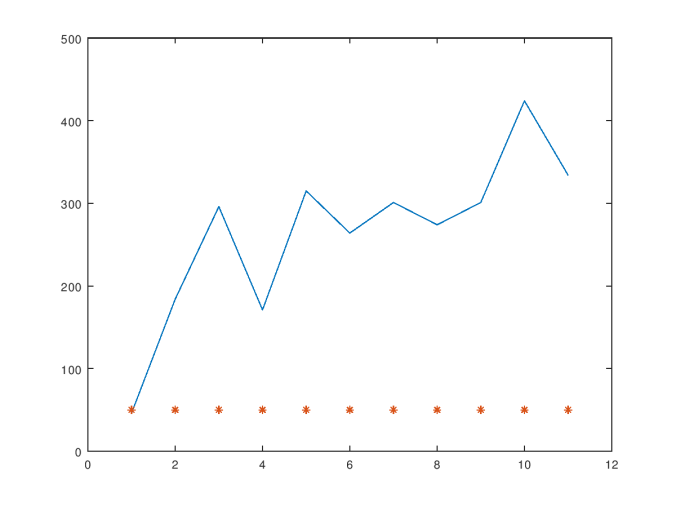
Note that as we decrease the value of adjustment, we decrease the difference between the sets of numbers generated by the two loops in the code above. As a result, decreasing the value of adjustment blurs the line between the two categories of numbers. This is reflected in the results produced by the algorithm, as shown in the attached graph, in which the number of categories decreases exponentially as the value of adjustment goes from 0 to 3.

adjustment

Similarly, as we increase spread, we increase the intersection between the two sets of numbers, thereby again decreasing the distinction between the two sets of numbers. However, the number of categories appears to grow linearly in this case as a function of spread over the interval .1 to .7, with adjustment fixed at 3.

spread

As a general matter, these results demonstrate that the algorithm behaves in an intuitive manner, generating a small number of wide categories when appropriate, and a large number of narrow categories when appropriate.

Generalizing this algorithm to the n-dimensional case should be straightforward, and I’ll follow up with those scripts sometime over the next few days. Specifically, we can simply substitute the arithmetic difference between two data points with the norm of the difference between two n-dimensional vectors. Of course, some spaces, such as an RGB color space, might require non-Euclidean measures of distance. Nonetheless, the point remains, that the concepts presented above are general, and should not, as a general matter, depend upon the dimension of the data set.

The relevant Octave / Matlab scripts are available here:

generate_linear_categories

generate_random_data

left_right_delta

optimize_linear_categories

partition_vec

spec_log

test_entropy_vec

vector_entropy